Show code cell source Hide code cell source

#Import libraries 
import numpy as np
import pandas as pd
import matplotlib.pyplot as plt
from sklearn.linear_model import LinearRegression
import matplotlib.animation as animation
from matplotlib.animation import FuncAnimation
from mpl_toolkits.mplot3d import axes3d

1.3. JNB Lab Solutions

1.3.1. Patterns in Nature

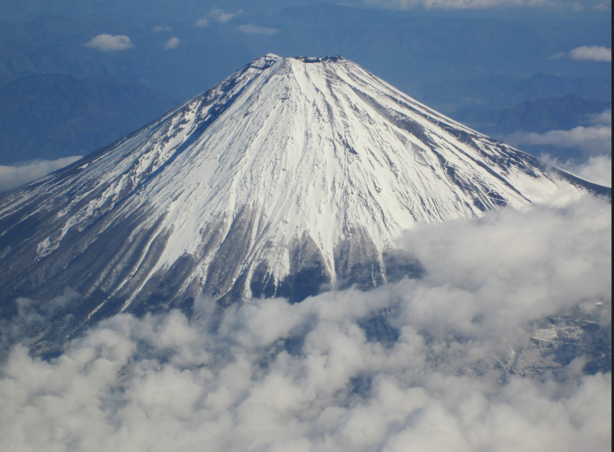
Solution to Exercise 1a

Show code cell source Hide code cell source

from IPython.display import Image
Image(filename='MtFuji.png',width=100,height=100)

Solution to Exercise 1b

Show code cell source Hide code cell source

from IPython.display import YouTubeVideo
YouTubeVideo('oYEtLQ3lEH0',width=200,height=200)

1.3.2. Patterns in Societal Data

Solution to Exercise 2

Show code cell source Hide code cell source

#STEP TWO
df2=raw_CPS_data[['address','student_count_total','student_count_black','graduation_rate_school','zip']]
df2=df2[df2["zip"]==60623]
df2=df2.dropna()
df2=df2.reset_index(drop=True) #rows are labelled 0,1,2,... 
print("Total number of CPS schools considered in 60623 is",len(df2["zip"])) #len = length
print("Largest student_count_total = ",df2["student_count_total"].max())
print("Smallest student_count_total = ",df2["student_count_total"].min())
df2.head(2)

Total number of CPS schools considered in 60623 is 9
Largest student_count_total =  559
Smallest student_count_total =  100

	address	student_count_total	student_count_black	graduation_rate_school	zip
0	2345 S CHRISTIANA AVE	559	66	68.9	60623
1	3120 S KOSTNER AVE	319	41	86.5	60623

Show code cell source Hide code cell source

#STEP THREE
df2.columns= ["address","total","black","graduate","zip"]
for i in df2.index:
    df2.loc[i,'%black']=round(100*df2.loc[i,'black']/df2.loc[i,'total'],1)
df2.head(2)

	address	total	black	graduate	zip	%black
0	2345 S CHRISTIANA AVE	559	66	68.9	60623	11.8
1	3120 S KOSTNER AVE	319	41	86.5	60623	12.9

Show code cell source Hide code cell source

#STEP FOUR
from sklearn.linear_model import LinearRegression #sklearn is a machine learning library
X=df2[["%black"]]
Y=df2[["graduate"]]
reg=LinearRegression()
reg.fit(X,Y)
print("Intercept is ", reg.intercept_)
print("Slope is ", reg.coef_)
print("R^2 for OLS is ", reg.score(X,Y))
# x values on the regression line will be between 0 and 100 with a spacing of .01
x = np.arange(0, 100 ,.01) 
# define the regression line y = mx+b here
[[m]]=reg.coef_
[b]=reg.intercept_
y =  m*x  + b   
# plot the school data
df2.plot(x='%black', y='graduate', style='o')  
plt.title('% Black vs %Graduate for 9 CPS Schools in 60623')  
plt.xlabel('% Black')  
plt.ylabel('% Graduate')  
# plot the regression line 
plt.plot(x,y, 'r') #add the color for red
plt.legend([],[], frameon=True)
plt.grid()
plt.savefig("CPSregression2.png")
plt.show()

Intercept is  [82.47649769]
Slope is  [[-0.14939133]]
R^2 for OLS is  0.429488206625943

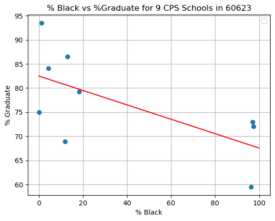
This shows graduates rates tend not to be as strong in the predominantly black schools in 60623.

1.3.3. Patterns in Mathematics

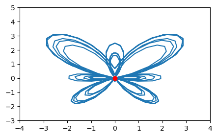
Solution to Exercise 3a

Show code cell source Hide code cell source

#Butterfly Curve
%matplotlib inline
#-----Set Up Plot -----
fig= plt.figure(figsize=(5,3))
plt.xlim(-4,4)
plt.ylim(-3,5)
##-----PARAMETRIC DEFINITION OF Butterfly CURVE------
t = np.arange(0, 12*np.pi, 0.1)
xt=np.sin(t)*(np.exp(np.cos(t))-2*np.cos(4*t)-(np.sin(t/12))**5)      
yt=np.cos(t)*(np.exp(np.cos(t))- 2*np.cos(4*t)-(np.sin(t/12))**5) 
plt.gca().plot(xt, yt)

def init():
    redDot, = plt.gca().plot([0], [0], 'ro') #starting position of dot
    return redDot,

def animate(i):
    redDot,= plt.gca().plot([np.sin(i)*(np.exp(np.cos(i))-2*np.cos(4*i)-(np.sin(i/12))**5) ], [np.cos(i)*(np.exp(np.cos(i))- 2*np.cos(4*i)-(np.sin(i/12))**5) ],'ro',ms=2,alpha=1)
    return redDot,

# create animation using the animate() function
ani = animation.FuncAnimation(fig, animate, frames=np.arange(0,12*np.pi,.01), init_func=init, interval=5, blit=True, repeat=False)

plt.show()

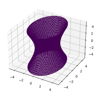
Solution to Exercise 3b.

def hyperboloid_1sheet(x,y,z):
    return (x/2)**2+(y/3)**2-(z/4)**2-1

plot_implicit(hyperboloid_1sheet)

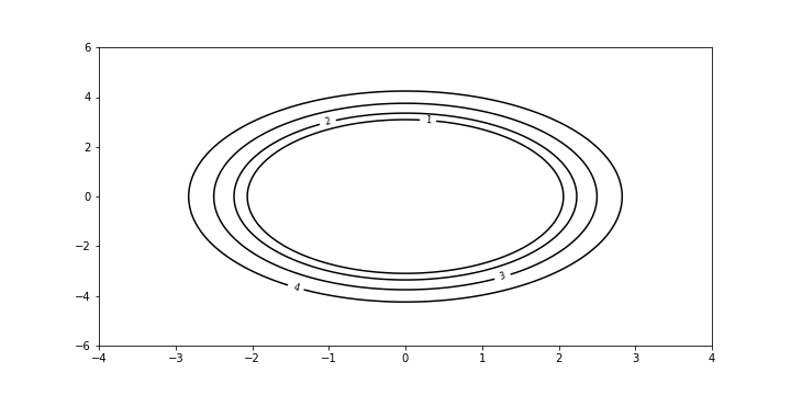
Show code cell source Hide code cell source

%matplotlib inline
plt.figure(figsize=(10,5))

#---Create grid points at which to evaluate the function z(x,y)
x = np.linspace(-4, 4, 250)
y = np.linspace(-6, 6, 250)
X, Y = np.meshgrid(x, y)
Z=4*np.sqrt((X/2)**2+(Y/3)**2-1)
#--Create the Contours--
contours=plt.contour(X, Y, Z, levels=np.linspace(0,4,5), colors='black');
#---Plot the Dividing Streamline---------
plt.clabel(contours, inline=True, fontsize=8)
plt.savefig('hyperb1.png')

1.3.4. Connecting Patterns in Mathematics to Patterns in Nature and Society

Solution to Exercise 4.

An ineffective system is one in which the two extraction wells (one mid-plume and one midstream) are not strong enough to capture all the pollution detected by the monitoring wells.

A regular system is one where the two extractions working together are sufficient to capture all the pollution.

An inefficient system is one where the mid-plume extraction well could be turned off, and the downstream extraction well by itself is sufficiently strong to capture all the pollution.