2.7. JNB LAB: After-School Program Demo

Note

One way to wrap-up an after-school program is to have the students do a combined presentation showing several things they learned throughout the program. It is a good idea to practice the presentations at least once or twice in advance.

Today our class will demonstrate several things which can be done with Jupyter Notebooks.

First we load standard libraries for analyzing and plotting data.

import numpy as np 
import pandas as pd 
import matplotlib as mpl
import matplotlib.pyplot as plt

2.7.1. DEMO 1: City of Chicago Budget

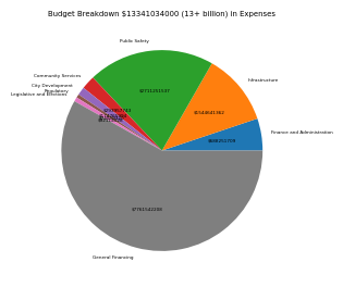
We will make a piechart of the City of Chicago budget.

1. First let’s look at the 2022 City of Chicago revenue details.

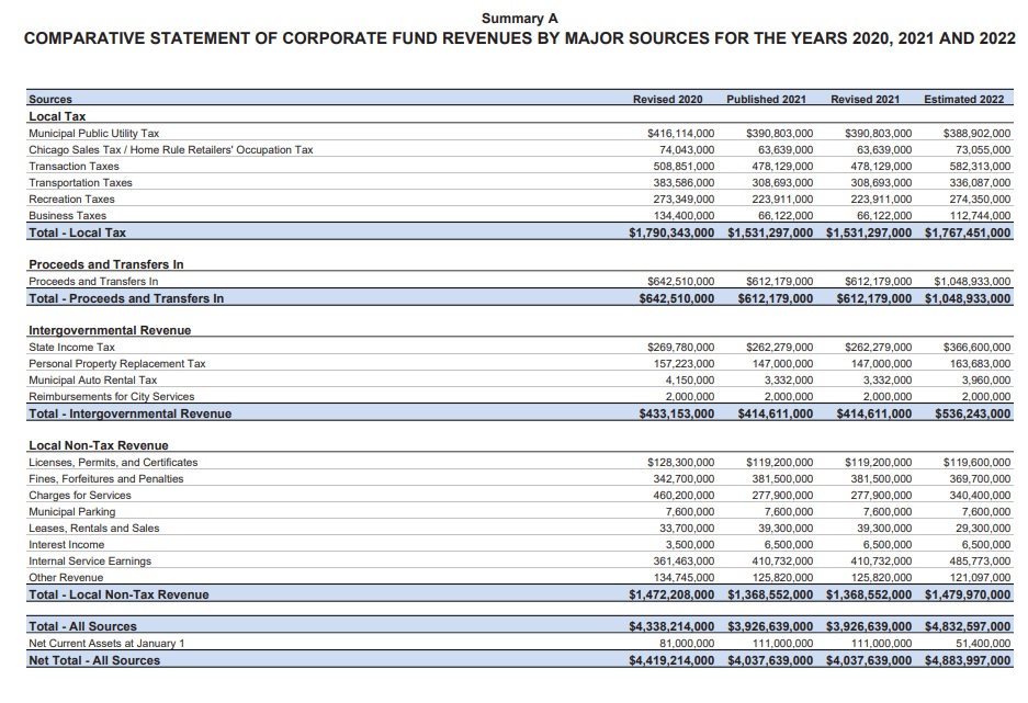
2. Next let’s read an Excel sheet with the summary of the 2023 budget.

budget=pd.read_excel('ChicagoBudget.xlsx')
budget

	EXPENSE	2023 BUDGET
0	Finance and Administration	688251735
1	Infrastructure	1544641397
2	Public Safety	2711251614
3	Community Services	293957760
4	City Development	174766005
5	Regulatory	74509317
6	Legislative and Elections	92114035
7	General Financing	7761542137

3. A pie chart will show us the proportions.

Show code cell source Hide code cell source

fig, ax = plt.subplots(figsize=(3,3)) #you can adjust the figsize  (5,5)=(length,width)
plt.rcParams['font.size'] = 3  #fontsize
budget_items = budget["EXPENSE"] #categories
budget_amounts = budget["2023 BUDGET"] #amounts
total=sum(budget_amounts)
ax=plt.pie(budget_amounts,labels=budget_items,autopct=lambda p: '${:.0f}'.format(p * total / 100)) #make pie chart  autopct='%1.0f%%'
plt.gca().set_title('Budget Breakdown $'+str(total)+' (13+ billion) in Expenses',size=5) #add a title
fig.savefig('Budget.png') #save the piechart to a file Budget.png

Exercise

Exercise

Enlarge the size of the piechart so it is easier to read. Make sure you enlarge the fontsize as well as the chart size.

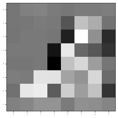
2.7.2. Demo 2 Pixel Images

We can increase the resolution of images by increasing the number of pixels.

Show code cell source Hide code cell source

# PACKAGE: DO NOT EDIT THIS CELL
%matplotlib inline
from ipywidgets import interact
import cv2, os

Show code cell source Hide code cell source

def makepixelimage(folder, N):

    directory = folder

    # A data structure called a dictionary is used to store the image data and the dataframes we'll make from them.
    imgs = {}
    dfs = {}

    # Specify the pixel image size 
    dsize = (N, N)

    # This will iterate over every image in the directory given, read it into data, and create a 
    # dataframe for it. Both the image data and its corresponding dataframe are stored.
    # Note that when being read into data, we interpret the image as grayscale. 
    pos = 0
    for filename in os.listdir(directory):
        f = os.path.join(directory, filename)
        # checking if it is a file
        if os.path.isfile(f):
            imgs[pos] = cv2.imread(f, 0) # image data
            imgs[pos] = cv2.resize(imgs[pos], dsize)
            dfs[pos] = pd.DataFrame(imgs[pos]) # dataframe
            pos += 1
    return plt.imshow(imgs[0], cmap="gray")

makepixelimage("images", 8)

<matplotlib.image.AxesImage at 0x18fccc85110>

Exercise

Increase the image resolution to 16x16 and then 32x32 so the image will become much clearer.

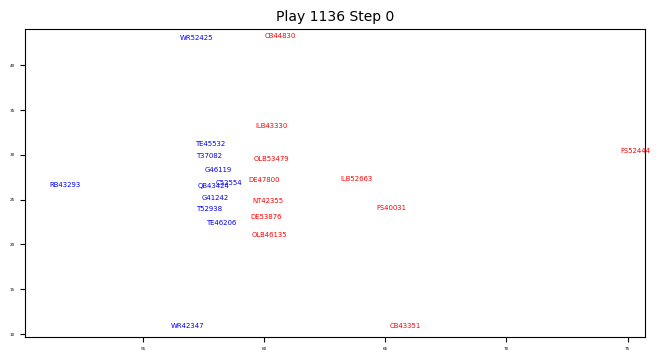
2.7.3. DEMO 3: Track NFL Player Positions

We will plot the movement of two players step by step in a given play Dataset: NFL_play.xlsx

1. Import special libraries.

Show code cell source Hide code cell source

import matplotlib.animation as animation
from matplotlib.animation import FuncAnimation

2. Read the Player Tracking Data

track_play=pd.read_excel('NFL_play.xlsx')
track_play.head(22)

	Unnamed: 0	game_play	game_key	play_id	nfl_player_id	datetime	step	team	position	jersey_number	x_position	y_position	speed	distance	direction	orientation	acceleration	sa
0	0	58580_001136	58580	1136	44830	2021-10-10T21:08:20.900Z	-108	away	CB	22	61.59	42.60	1.11	0.11	320.33	263.93	0.71	-0.64
1	1	58580_001136	58580	1136	42355	2021-10-10T21:08:20.900Z	-108	away	NT	75	59.63	24.33	0.10	0.01	7.98	227.03	0.41	0.27
2	2	58580_001136	58580	1136	43330	2021-10-10T21:08:20.900Z	-108	away	ILB	55	60.67	30.89	3.19	0.32	334.89	303.31	1.95	-1.73
3	3	58580_001136	58580	1136	52425	2021-10-10T21:08:20.900Z	-108	home	WR	88	56.59	42.86	0.13	0.01	158.78	98.31	0.32	0.02
4	4	58580_001136	58580	1136	43293	2021-10-10T21:08:20.900Z	-108	home	RB	21	51.11	26.42	0.14	0.01	144.58	78.52	0.52	0.51
5	5	58580_001136	58580	1136	40031	2021-10-10T21:08:20.900Z	-108	away	FS	23	70.53	22.03	0.32	0.03	285.68	287.44	0.28	0.27
6	6	58580_001136	58580	1136	41242	2021-10-10T21:08:20.900Z	-108	home	G	70	57.33	24.80	0.03	0.01	328.04	57.38	0.07	0.07
7	7	58580_001136	58580	1136	52938	2021-10-10T21:08:20.900Z	-108	home	T	78	57.27	23.47	0.19	0.02	356.50	87.29	0.10	-0.10
8	8	58580_001136	58580	1136	42347	2021-10-10T21:08:20.900Z	-108	home	WR	19	56.23	10.68	0.07	0.01	132.91	123.39	0.19	-0.14
9	9	58580_001136	58580	1136	46135	2021-10-10T21:08:20.900Z	-108	away	OLB	59	59.90	21.14	1.58	0.16	218.10	278.39	0.48	0.22
10	10	58580_001136	58580	1136	43424	2021-10-10T21:08:20.900Z	-108	home	QB	4	57.31	26.27	0.07	0.01	207.25	93.25	0.11	0.07
11	11	58580_001136	58580	1136	43351	2021-10-10T21:08:20.900Z	-108	away	CB	24	64.39	10.89	0.80	0.08	130.49	309.04	0.44	-0.44
12	12	58580_001136	58580	1136	45532	2021-10-10T21:08:20.900Z	-108	home	TE	89	57.16	30.99	0.07	0.01	39.61	100.73	0.51	-0.14
13	13	58580_001136	58580	1136	46119	2021-10-10T21:08:20.900Z	-108	home	G	52	57.36	28.02	0.08	0.01	127.21	241.42	0.05	0.04
14	14	58580_001136	58580	1136	37082	2021-10-10T21:08:20.900Z	-108	home	T	77	57.16	29.54	0.12	0.01	145.27	85.16	0.07	0.01
15	15	58580_001136	58580	1136	53876	2021-10-10T21:08:20.900Z	-108	away	DE	91	59.65	22.71	0.23	0.02	268.69	271.27	0.23	-0.23
16	16	58580_001136	58580	1136	53479	2021-10-10T21:08:20.900Z	-108	away	OLB	51	59.47	29.52	0.24	0.02	296.78	257.94	1.12	0.26
17	17	58580_001136	58580	1136	52663	2021-10-10T21:08:20.900Z	-108	away	ILB	48	63.25	27.50	0.51	0.05	183.62	253.71	0.31	0.31
18	18	58580_001136	58580	1136	46206	2021-10-10T21:08:20.900Z	-108	home	TE	86	57.37	22.12	0.37	0.04	127.85	63.63	0.69	0.62
19	19	58580_001136	58580	1136	52444	2021-10-10T21:08:20.900Z	-108	away	FS	29	72.19	31.46	0.61	0.06	11.77	247.69	0.63	-0.33
20	20	58580_001136	58580	1136	47800	2021-10-10T21:08:20.900Z	-108	away	DE	97	59.48	26.81	0.23	0.01	346.84	247.16	1.29	0.90
21	21	58580_001136	58580	1136	52554	2021-10-10T21:08:20.900Z	-108	home	C	63	58.18	26.52	0.16	0.02	357.62	102.55	0.60	0.58

3. Plot the positions of the players at step -108 (before the snap) of play 1136.

Show code cell source Hide code cell source

fig= plt.figure(figsize=(8,4))
temp=track_play[track_play["step"]==0]
xmin=temp["x_position"].min()
xmax=temp["x_position"].max()
ymin=temp["y_position"].min()
ymax=temp["y_position"].max()
plt.xlim(xmin-1,xmax+1)
plt.ylim(ymin-1,ymax+1)
for i in temp.index:
    x=temp.loc[i,"x_position"]
    y=temp.loc[i,"y_position"]
    n=temp.loc[i,"nfl_player_id"]
    p=temp.loc[i,"position"]
    if temp.loc[i,"team"]=='home':
        plt.text(x, y, p+str(n),color='b',size=5)
    else:
        plt.text(x, y, p+str(n),color='r',size=5)
plt.title("Play 1136 Step 0",size=10)
plt.show()

4. Let’s define a function which creates a snapshot of the position of the players at any step of a given play.

Show code cell source Hide code cell source

def teampositions(data,play,step):
    playdf=data[data["play_id"]==play]
    playdf = playdf.sort_values(by = 'step')
    playdf=playdf.reset_index(drop=True)
    stepdf=playdf[playdf["step"]==step]
    xmin=stepdf["x_position"].min()
    xmax=stepdf["x_position"].max()
    ymin=stepdf["y_position"].min()
    ymax=stepdf["y_position"].max()
    fig= plt.figure(figsize=(8,4))
    plt.xlim(xmin-1,xmax+1)
    plt.ylim(ymin-1,ymax+1)
    for i in stepdf.index:
        x=stepdf.loc[i,"x_position"]
        y=stepdf.loc[i,"y_position"]
        n=stepdf.loc[i,"nfl_player_id"]
        p=stepdf.loc[i,"position"]
        if stepdf.loc[i,"team"]=='home':
            plt.text(x, y, p,color='b',size=5)
        else:
            plt.text(x, y, p,color='r',size=5)
    plt.title("Play"+str(play)+ "  Step"+str(step),size=10)
    plt.savefig(str(step)+'.png')
    return

5. Let’s use this function to create snapshots of player positions for the first 50 steps after the snap of play 1136.

Show code cell source Hide code cell source

frames=50
for step in np.arange(0,frames,1):
    teampositions(track_play,1136,step)
    

6. Let’s combine these snapshots into an animation. Can you figure out what happened on this play?

Show code cell source Hide code cell source

from PIL import Image
images = []
for n in range(frames):
    exec('a'+str(n)+'=Image.open("'+str(n)+'.png")')
    images.append(eval('a'+str(n)))
images[0].save('play.gif',
               save_all=True,
               append_images=images[1:],
               duration=5,
               loop=0)

Exercise

Exercise

Create a video which isolates the movement of just two players: the wide receiver (52425) and cornerback (44830) at the top of the screen.

2.7.4. Demo 4 Word Clouds

Let’s make a word cloud Christmas card using the song “Twelve Days of Christmas.”

import wordcloud

Show code cell source Hide code cell source

#Define a function which counts the interesting words
def calculate_frequencies(textfile):
    #list of punctuations
    punctuations = '''!()-[]{};:'"\,<>./?@#$%^&*_~'''
    #list of uninteresting words 
    uninteresting_words = ["AND","BY","IT","THE","THAT","A","IS","HAD","TO","NOT","BUT","FOR","OF","WHICH","IF","IN","ON","WERE","YE","THOU"]
    
     # removes punctuation and uninteresting words
    import re
    fc1=str(textfile)
    fc2= fc1.split(' ')
    for i in range(len(fc2)): 
        fc2[i] = fc2[i].upper()
    #Remove punctuations
    fc3 = []
    for s in fc2:
        if not any([o in s for o in punctuations]):
            fc3.append(s)
    #Remove uninteresting words
    fc4=[]
    for s in fc3:
        if not any([o in s for o in uninteresting_words]):
            fc4.append(s)
    fc5=[]
    for s in fc4:
        if not any([o.lower() in s for o in uninteresting_words]):
            fc5.append(s)
            
    while('' in fc5) : 
        fc5.remove('') 
        
    import collections
    fc6 = collections.Counter(fc5)

    #wordcloud
    cloud = wordcloud.WordCloud( max_words = 12)  #can adjust the number of words
    cloud.generate_from_frequencies(fc6)
    return cloud.to_array()

#Open the text file with the words to be plotted.
with open('twelvedays.txt','r') as file:  
    carol = file.readlines()
    
#make the wordcloud   
carol = calculate_frequencies(carol)
plt.imshow(carol, interpolation = 'nearest')
plt.axis('off')
plt.savefig('card.png', bbox_inches='tight')  

Exercise

Exercise

Add the words “Merry Christmas!” in red onto the middle of the wordcloud.

Demo 5 Name that Tune

1. Musical sound waves are created by rapid vibrations caused by musical isntruments.

from IPython.display import YouTubeVideo
YouTubeVideo('tVYQRC1-D54')

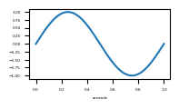
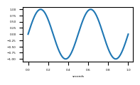
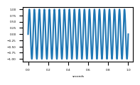
2. Sound waves are represented mathematically by sine waves with different frequencies.

def sinewave(frequency):
    #-----------CREATE THE SOUND WAVE-------------------
    sampling_rate=44100  #how many times we take a measurement each second
    t = np.linspace(0,1,sampling_rate)  # take 44100 samples in 1 second; 
    sound_wave=np.sin(frequency* 2*np.pi* t)  # mathematical definition of a sine wave
    #----------PLOT THE SOUND WAVE----------------------
    import matplotlib.pyplot as plt
    fig=plt.figure(figsize=(2,1))
    plt.plot(t,sound_wave)
    plt.xlabel("seconds")
    return

sinewave(1)  #frequency=1 and 1 cycle per second

sinewave(2)  #frequency=2 and 2 cycles per second

sinewave(20) #frequency=20 and 20 cycles per second

3. A computer can create a musical tone based on a given frequency.

def play(freq):
    import numpy as np
    from IPython.display import Audio  #library used to create sounds
    sampling_rate = 44100 # <- rate of sampling
    t = np.linspace(0, 2,  sampling_rate) # <- setup time values
    sound_wave = np.sin(2 * np.pi * freq * t) # <- sine function formula
    return Audio(sound_wave, rate=sampling_rate, autoplay=True) # play the generated sound

play(220) # play a sound at 220 hz 

4. A musical scale is a sequence of frequencies.

from IPython.display import Audio 
rest=0
do=220
re=9/8*220
mi=5/4*220
fa=4/3*220
so=3/2*220
la=5/3*220
ti=15/8*220
do1=2*220
re1=2*9/8*220
mi1=2*5/4*220
fa1=2*4/3*220
so1=2*3/2*220
la1=2*5/3*220
ti1=2*15/8*220
do2=2*2*220
scale=[do,re,mi,fa,so,la,ti,do1]

def play(song):
    song=np.array(song)
    framerate = 44100
    t = np.linspace(0, len(song) / 2, round(framerate * len(song) / 2))[:-1]
    song_idx = np.floor(t * 2).astype(int)
    data = np.sin(2 * np.pi * song[song_idx] * t)
    return Audio(data, rate=framerate, autoplay=True)
play(scale)

5. Can you name that tune?

tune= [so, so , la, la, so, fa,mi,rest,so, so , la, la, so, fa,mi,rest,so,so,la,ti,do1,do1,re1,re1,ti,la,ti,la,so,so,la,ti,do1,do1,ti,la,so,so,rest,rest,la,la,so,fa,mi,mi,rest,rest,so,so,do,fa,mi,mi,re,re,do,do,do,do,rest,rest]
play(tune)

from IPython.display import YouTubeVideo
YouTubeVideo('L4PA-MFSM34')

Exercise

Exercise

Demonstrate how to create a new tune.