import matplotlib.pyplot as plt
import numpy as np
9.2. Linear Systems#
9.2.1. Systems of Linear Equations#
This section introduces systems of linear equations, or linear systems, and discusses how to find their solutions.
Linear Systems#
A linear equation in \(n\) variables is an equation of the form:
where \(x_1, x_2, \dots, x_n\) are variables, and \(b\) and the coefficients \(a_1, a_2, \dots, a_n\) are real numbers. A system of linear equations is a collection of linear equations in the same set of variables. For example, a system of \(m\) equations in \(n\) variables \(x_1, x_2, \dots, x_n\) can be represented as:
A solution for a linear system is a list of real numbers \((s_1, s_2, \dots, s_n)\) that satisfy each equation in the system. Two linear systems are said to be equivalent if they have the same set of solutions. In other words, every solution of the first system is also a solution of the second system, and vice versa. Furthermore, a linear system is called consistent if it has solutions; otherwise, it is called inconsistent. It turns out that any linear system has either no solutions, exactly one solution, or infinitely many solutions.
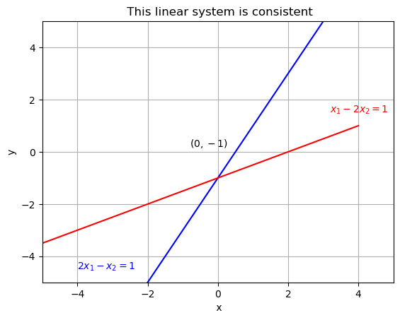
As an example, let’s consider a simple case where we have two equations in two unknowns. Finding the solution of such a system is easy as it comes down to finding the intersection of two lines in the plane. More precisely, the graph of each equation in this system represents a line, and a point \((s_1, s_2) \in \mathbb{R}^2\) is a solution if and only if it lies on both lines.
Example 1
The following system is consistent, and its only solution is \((0, -1)\).
The following cell plots the graph of these lines on the same plane:
Show code cell source
# Data for plotting

x = range(-5, 5)
y1 = [ 2*k-1 for k in x]
y2 = [ (k-2)/2 for k in x]

fig, ax = plt.subplots()

# Specify the length of each axis
ax.set_xlim(-5,5)
ax.set_ylim(-5,5)

#Plot x and y1 using blue color
ax.plot(x, y1, color = 'b')
ax.text(-4,-4.5,'$2x_1 - x_2 = 1$', color = 'b')

#Plot x and y2 using red color
ax.plot(x, y2, color = 'r')
ax.text(3.2,1.5,'$x_1 -2x_2 = 1$', color = 'r')

# add label to the intersection
ax.text(-0.8, 0.2, '$(0,-1) $' )

# Add labels and a title to the graph
ax.set(xlabel=' x', ylabel='y',
       title=' This linear system is consistent')
ax.grid()

plt.show()
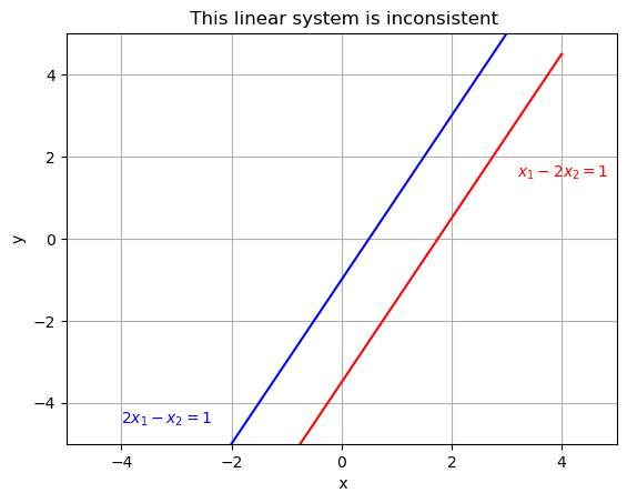
(2) The next system is inconsistent because it does not have any solutions.
Show code cell source
import matplotlib.pyplot as plt

# Data for plotting

x = range(-5, 5)
y1 = [ 2*k-1 for k in x]
y2 = [ 2*k-7/2 for k in x]

fig, ax = plt.subplots()

# Specify the length of each axis
ax.set_xlim(-5,5)
ax.set_ylim(-5,5)

#Plot x and y1 using blue color
ax.plot(x, y1, color = 'b')
ax.text(-4,-4.5,'$2x_1 - x_2 = 1$', color = 'b')

#Plot x and y2 using red color
ax.plot(x, y2, color = 'r')
ax.text(3.2,1.5,'$x_1 -2x_2 = 1$', color = 'r')


# Add labels and a title to the graph
ax.set(xlabel=' x', ylabel='y',
       title=' This linear system is inconsistent')
ax.grid()

plt.show()
Similarly, we can find a linear system containing two equations in two unknowns that has infinitely many solutions (see Exercise 1).
9.2.2. Solving a Linear System#
A fundamental question about a linear system is whether or not it is consistent and, if it is, whether it has a unique solution or infinitely many solutions. To that end, we utilize the row reduction algorithm. The main idea is to use a set of operations called elementary row operations to convert a system into an equivalent system that is easier to solve. These elementary row operations are:
Swapping two equations
Multiplying an equation by a nonzero number
Adding a multiple of one equation to another equation
To do this, we first represent the essential information of a system in a compact rectangular form called the augmented matrix of the system. For example, the augmented matrix of the system:
is the following matrix:
In the augmented matrix, each row represents an equation in the system. We can define the same operations for matrices, by simply replacing “equation” with “row” in their definitions. Moreover, we say that two matrices A and B are row equivalent if one can be transformed into the other using the elementary row operations mentioned above.
The goal is to convert the augmented matrix to another matrix form that is easier to solve. This easier form is called echelon form. This new matrix form corresponds to a linear system that is simpler to deal with and is equivalent to the original system.
To formally define the echelon form, we need to introduce the following concepts:
Zero Row: a row containing only zero entries.
Leading Entry: the leftmost nonzero entry in a nonzero row.
A rectangular matrix is in row echelon form (REF) if:
All non-zero rows are above any zero row
Every leading term of a row is in a column to the right of the leading entry
Entries below a leading entry are zero
A rectangular matrix is in reduced row echelon form (RREF) if:
It is in echelon form
Every leading entry is 1
Entries above a leading entry are zero
Example 2
The following matrix is in REF. The leading entries (\(\blacksquare\)) can be any nonzero real numbers, while the (\(*\)s) may be any real number.
The following matrix is in RREF:
Theorem 1
Any nonzero matrix is row equivalent to one and only one matrix in RREF.
Reduction Algorithm:
The reduction algorithm takes in a matrix and produces a matrix in RREF. It consists of 5 steps; in step four, it produces a matrix in REF, and in the fifth step, RREF. We will show the algorithm with an example:
Example 3
Find the RREF of
We represent a matrix as a numpy array
#numpy array to represent a matrix: each row is a list.
A = np.array([[0,2,3,9],[2,-1,1,8],[3,0,-1,3]])
A
array([[ 0,  2,  3,  9],
       [ 2, -1,  1,  8],
       [ 3,  0, -1,  3]])
Lets write Pythons functions that perform the row operations:
Show code cell source
# Swap two rows

def swap(matrix, row1, row2):

    copy_matrix = np.copy(matrix).astype('float64')

    copy_matrix[row1,:] = matrix[row2,:]
    copy_matrix[row2,:] = matrix[row1,:]

    return copy_matrix


# Multiple all entries in a row by a nonzero number


def scale(matrix, row, scalar):
    copy_matrix=np.copy(matrix).astype('float64')
    copy_matrix[row,:] = scalar*matrix[row,:]
    return copy_matrix

# Replacing row 1 by the sum of itself and a multiple of row2

def replace(matrix, row1, row2, scalar):
    copy_matrix = np.copy(matrix).astype('float64')
    copy_matrix[row1] = matrix[row1] + scalar * matrix[row2]
    return copy_matrix
Step 1: Start with the leftmost nonzero entry in the first column and bring it to the top row. This is a pivot column; the pivot position should be on top.
Show code cell source
#the leftmost nonzero column:
A[:,0]
array([0, 2, 3])
Step 2: Select a nonzero entry in the pivot column as a pivot. If necessary, swap the rows to move this entry to the top.
Show code cell source
#The first nonzero element is at row 2. Swap the rows 1 and 2:
A1 = swap(A, 0, 1)
A1
array([[ 2., -1.,  1.,  8.],
       [ 0.,  2.,  3.,  9.],
       [ 3.,  0., -1.,  3.]])
Step 3: Use scaling operation to make the pivot 1, and replacement operation to create zeros below the leading 1:
Show code cell source
#Divide row1 by 2
A2 = scale(A1, 0, 1/2)
A2

#Replace row3  by row3-3*row1

A3 = replace(A2,2,0,-3)
A3
array([[ 1. , -0.5,  0.5,  4. ],
       [ 0. ,  2. ,  3. ,  9. ],
       [ 0. ,  1.5, -2.5, -9. ]])
Step 4: Ignore the row with a pivot position and cover all rows, if any, above it. For the remaining matrix, apply steps 1-3. Repeat the process until there are no more non-zero rows to modify.
Show code cell source
#Divide row2 by 2
A4 = scale(A3, 1, 1/2)
A4

#Replace row3  by row3-3*row1

A5 = replace(A4, 2, 1, -1.5)
A5
array([[  1.  ,  -0.5 ,   0.5 ,   4.  ],
       [  0.  ,   1.  ,   1.5 ,   4.5 ],
       [  0.  ,   0.  ,  -4.75, -15.75]])
We apply the fifth step to get the RREF:
Step 5: If a pivot is not one, we use the scaling operation to make it one. Moreover, we create zeros above each pivot starting with the rightmost pivot and work upward and to the left.
Show code cell source
#make all entries in pivot positions 1
A6 = scale(A5,2, 1/-4.75)
A6

#replace row1 by row1 + 0.5* row 2
A7 = replace(A6, 0, 1, 0.5)
A7

#replace row1 by row1 - 1.25* row 2
A8 = replace(A7, 0, 2, -1.25)
A8

#replace row2 by row2 - 1.5* row 3
A9 = replace(A8,1,2,-1.5)
A9
array([[ 1.        ,  0.        ,  0.        ,  2.10526316],
       [ 0.        ,  1.        ,  0.        , -0.47368421],
       [-0.        , -0.        ,  1.        ,  3.31578947]])
\(A_9\) is the RREF of \(A\), and the augmented column (the rightmost column) of \(A_9\) is the solution to the original system.
Example 4
Find the solution set of the following system of equations:
Solution: Let’s set up the augmented matrix of the system and then convert it to its RREF:
Show code cell source
#The augmented matrix
R = np.array([[2,-5, 1, 2], [1,-1,0,4], [3,0,-1,3]])
R

#finding the first pivot entry: 1
R1= swap(R, 1, 0)
R1

#making entries below 1 zero
R2 = replace(R1, 1, 0, -2)
R2

R3 = replace(R2, 2,0, -3)
R3

#making entries below the second pivot entry (-3) zero
R4 = replace(R3, 2, 1, 1)
R4
array([[  1.,  -1.,   0.,   4.],
       [  0.,  -3.,   1.,  -6.],
       [  0.,   0.,   0., -15.]])
R4 is in REF. Now we write back the corresponding linear system:
The last equation is impossible, which means the system is inconsistent.
Exercises#
Exercises
Find a linear system containing two equations in two unknowns that has infinitely many solutions. Verify your answer by plotting the lines of these equations on the same plane.
Find a linear system that is equivalent to the linear system in Example 1.
Determine which of the following matrices are in REF. For those that are, identify their pivot columns. Are any in RREF?
\(A = \begin{bmatrix} 0 & 0 & 4 &-1 && 0\\ 0 & 0 & 0 &0 && 0 \\ 0 & 0& 0 & 0 &&3\end{bmatrix}\)
\(B = \begin{bmatrix} 1 & 1 & 0 && 1\\ 0 & 1 & 1 &&0\\ 0 & 0 & 1 &&1 \end{bmatrix}\)
\(C = \begin{bmatrix} 1 & 0 & 3 && 0\\ 0 & 1 & 0 &&0\\ 0 & 0 & 0 &&1 \end{bmatrix}\)
For the above matrices write the corresponding linear systems and find their solutions.
Find the REF of \(D = \begin{bmatrix} 0 & 1 & 2\\ 1 & 0 & 3\\ 4 & -3 & 8 \end{bmatrix}\).
9.2.3. Matrix Equation.#
Note
Linear systems can be represented by equations involving vectors and matrices. In this section, we use such representations to study and analyze linear systems.
Let \(n\) be a positive integer, and \(\mathbb{R}^n\) be the collection of all ordered \(n\)-tuples of real numbers. An element of \(\mathbb{R}^n\), denoted by an \(n\times 1\) column matrix, and is called a vector. For example,
A vector whose entries are all zero is called the zero vector and is denoted by \(\vec{0}\). When there is no risk of confusion we sometimes omit the arrow and use simply \(0\)
Two vectors \(\vec{u} = \begin{bmatrix} u_1 \\ u_2 \\ \vdots \\ u_n \end{bmatrix}\) and \(\vec{v} = \begin{bmatrix} v_1 \\ v_2 \\ \vdots \\ v_n \end{bmatrix}\) are equal if their corresponding entries are equal, that is if \(u_i = v_i\) for all \(i \leq n\).
Given a vector \(\vec{u} = \begin{bmatrix} u_1 \\ u_2 \\ \vdots \\ u_n \end{bmatrix}\) and a real number \(c\), the scalar product of \(\vec{u}\) by \(c\) is given by:
Theorem 2
Suppose \(\vec{u}\), \(\vec{v}\), \(\vec{w}\) are in \(\mathbb{R}^n\), and \(c\) and \(d\) are real numbers:
\(\vec{u} + \vec{v} = \vec{v} + \vec{u}\)
\((\vec{u} + \vec{v}) + \vec{w} = \vec{u} + (\vec{v} + \vec{w})\)
\(\vec{u} + \vec{0} = \vec{0} + \vec{u} = \vec{u}\)
\(\vec{u} + (-\vec{u}) = \vec{0}\)
\(c(\vec{u} + \vec{v}) = c\vec{u} + c\vec{v}\)
\((c+d)\vec{u} = c\vec{u} + d\vec{u}\)
\(c(d\vec{u}) = (cd)\vec{u}\)
Vector Equation#
A vector \(\vec{y} \in \mathbb{R}^n\) is called a linear combination of some vectors \(\vec{u_1}, \vec{u_2}, \dots, \vec{u_p} \in \mathbb{R}^n\), if there are real numbers \(c_1, c_2, \dots, c_p\) such that
The span of vectors \(\vec{u_1}, \vec{u_2}, \dots, \vec{u_p}\), denoted by \(span\ (\vec{u_1}, \vec{u_2}, \dots, \vec{u_p})\), is the set of all possible linear combinations:
In other words, the span represents all the vectors that can be formed by scaling and adding the given vectors \(\vec{u_1}, \vec{u_2}, \dots, \vec{u_p}\).
Example 1
Let \(\vec{y}=\begin{bmatrix} 7 \\ -4 \\3 \end{bmatrix}\), \(\vec{u}= \begin{bmatrix} 2 \\ -3\\-5 \end{bmatrix}\), and \(\vec{v} =\begin{bmatrix} 0 \\ 0 \\1 \end{bmatrix}\).
a. Compute \(2 \vec{u} - 3 \vec{v}\). b. Determine if \(\vec{y}\) is a linear combination of \(\vec{u}\) and \(\vec{v}\).
Solution:
(a).
Let’s use Python to double check our solution. A vector is a numpy array of a list.
Show code cell source
y = np.array([[7,-4,3]])
print("y = ", y)

u=np.array([[2,-3,-5]])
print("u = ", u)

v=np.array([[0,0,1]])
print("v = ", v)
y =  [[ 7 -4  3]]
u =  [[ 2 -3 -5]]
v =  [[0 0 1]]
Show code cell source
#(a). Compute 2u-3v

2*u+3*v
array([[ 4, -6, -7]])
(b). To determine if \(\vec{y}\) is a linear combination of \(\vec{u}\) and \(\vec{v}\), we need to check if there exists real numbers \(c_1\) and \(c_2\) such that:
Substituting the given values, we have:
Which is the same as:
or
This equation cannot be satisfied because there are no values of \(c_1\) and \(c_2\) that can make the left-hand side equal to the right-hand side. Therefore, \(\vec{y}\) is not a linear combination of \(\vec{u}\) and \(\vec{v}\).
In Example 1b), to solve a vector equation we converted it into a linear system. In general, the vector equation
has the same solution set as the linear system whose augmented matrix is
Note that for brevity, we represented the augmented matrix by its columns.
An indexed set of vectors \(\{\vec{v_1}, \vec{v_2}, \dots \vec{v_p}\}\) in \(\mathbb{R}^n\) is called a linearly independent set if the vector equation:
has only the trivial solution. The set is called linearly dependent if there are real numbers \(c_1,c_2, \dots c_p\), not all zero, such that
Theorem 3
A set of vectors containing the zero vector is linearly dependent.
A set of two vectors is linearly dependent if and only if one is a multiple of the other.
Example 2
Determine if the following vectors form a linearly independent set:
Solution:
We convert the augmented matrix in \((*)\) into its REF:
A = np.array([[1,4,7, 0], [2,5,8,0], [3,6,9,0]])
A
array([[1, 4, 7, 0],
       [2, 5, 8, 0],
       [3, 6, 9, 0]])
# Swap two rows

def swap(matrix, row1, row2):

    copy_matrix=np.copy(matrix).astype('float64')

    copy_matrix[row1,:] = matrix[row2,:]
    copy_matrix[row2,:] = matrix[row1,:]

    return copy_matrix


# Multiple all entries in a row by a nonzero number


def scale(matrix, row, scalar):
    copy_matrix=np.copy(matrix).astype('float64')
    copy_matrix[row,:] = scalar*matrix[row,:]
    return copy_matrix

# Replacing a row1 by the sum of itself and a multiple of row2

def replace(matrix, row1, row2, scalar):
    copy_matrix=np.copy(matrix).astype('float64')
    copy_matrix[row1] = matrix[row1]+ scalar * matrix[row2]
    return copy_matrix
A1 = replace(A, 1, 0, -2)
A1
array([[ 1.,  4.,  7.,  0.],
       [ 0., -3., -6.,  0.],
       [ 3.,  6.,  9.,  0.]])
A2 = replace(A1, 2, 0, -3)
A2
array([[  1.,   4.,   7.,   0.],
       [  0.,  -3.,  -6.,   0.],
       [  0.,  -6., -12.,   0.]])
A3 = replace(A2, 2, 1, -2)
A3
array([[ 1.,  4.,  7.,  0.],
       [ 0., -3., -6.,  0.],
       [ 0.,  0.,  0.,  0.]])
A4 = scale(A3, 1, -1/3)
A4
array([[ 1.,  4.,  7.,  0.],
       [-0.,  1.,  2., -0.],
       [ 0.,  0.,  0.,  0.]])
Writing this matrix as a linear system, we have
From this, it is clear that \(\{\vec{u}, \vec{v}, \vec{w}\}\) is not linearly independent because for any nonzero choice of \(z\), we get a non-trivial solution. For example, if \(z= 1\), then \(( -5, -2 , 1)\) is a non-trivial solution.
Matrix Equation \(A\vec{x}=\vec{b}\)#
Similarly, we can translate a linear system into a matrix equation of the form \(A\vec{x} = \vec{b}\). To that end, we need to define the product on the left-hand side of equality.
Let A be an \(m\times n\) matrix (a rectangular array) with columns \(\vec{a_1}, \vec{a_2}, \dots, \vec{a_n}\), and \(\vec{x}\in \mathbb{R}^n\). We can define the product of \(A\) and \(\vec{x}\), denoted by \(A\vec{x}\), as the linear combination of the columns of \(A\) where the coefficients are the components of \(\vec{x}\):
Note that \(A\vec{x}\) is defined only if the number of columns of A equals the number of entries of \(\vec{x}\)
Theorem 4 (properties of the product of A and \(\vec{x}\))
Suppose \(A\) is an \(m\times n\) matrix, \(\vec{u}\) and \(\vec{v}\) are in \(\mathbb{R}^n\) and \(c\) is a scalar. Then
\(A(\vec{u}+ \vec{v})= A \vec{u} + A \vec{v}\)
\(A(c\vec{u})= c A\vec{u}\)
Now let us discuss how to represent a linear system by a matrix equation. Consider:
and let
and \(\ \vec{x}= \begin{bmatrix} x_1 \\ x_2\\ \vdots \\ x_n \end{bmatrix}\ \) and \(\ \vec{b}= \begin{bmatrix} b_1 \\ b_2\\ \vdots \\ b_m \end{bmatrix}\ \). The matrix A is called the coefficient matrix. Then we can rewrite the above linear system as: \(A\vec{x}=\vec{b}.\) The next theorem describes when a matrix equation has at least one solution.
Theorem 5
Let \(A\) be an \(m\times n\) matrix. The following statements are logically equivalent:
For any \(\vec{b}\in \mathbb{R}^m\), the equation \(A\vec{x}=\vec{b}\) has a solution.
Each \(\vec{b}\in \mathbb{R}^m\) is a linear combination of columns of \(A\)
The columns of \(A\) span \(\mathbb{R}^m\)
A has a pivot position in every row.
Example 3
Let \(A\) be a matrix whose columns are \(\vec{u}\), \(\vec{v}\), \(\vec{w}\) from Example 2. Find vectors \(\vec{b}, \vec{c} \in \mathbb{R}^3\) such that \(A\vec{x}=\vec{b}\) has a solution and \(A\vec{x}=\vec{c}\) does not.
Solution:
Let
Now, let’s form the augmented matrix of equation \(A\vec{x}=\vec{b}\):
Now we can perform row operations to verify that it has a solution:
Ab = np.array([[1,4,7,1],[2,5,8,2],[3,6,9,3]])
Ab
array([[1, 4, 7, 1],
       [2, 5, 8, 2],
       [3, 6, 9, 3]])
B1 = replace(Ab, 1 , 0, -2)
B1
array([[ 1.,  4.,  7.,  1.],
       [ 0., -3., -6.,  0.],
       [ 3.,  6.,  9.,  3.]])
B2 = replace(B1, 2 , 0, -3)
B2
array([[  1.,   4.,   7.,   1.],
       [  0.,  -3.,  -6.,   0.],
       [  0.,  -6., -12.,   0.]])
B3 = replace(B2, 2, 1 , -2)
B3
array([[ 1.,  4.,  7.,  1.],
       [ 0., -3., -6.,  0.],
       [ 0.,  0.,  0.,  0.]])
B4 = scale(B3, 1 , -1/3)
B4
array([[ 1.,  4.,  7.,  1.],
       [-0.,  1.,  2., -0.],
       [ 0.,  0.,  0.,  0.]])
From this we see that for any \(z \in \mathbb{R}\) we have a unique solution. For example if \(z = 0\)
So the equation \(A\vec{x}=\vec{b}\) has a solution.
Now, we solve the equation \(A\vec{x}=\vec{c}\) to verify that it does not have a solution. Let’s form the augmented matrix \([A|\vec{c}]\):
Now we can perform row operations to verify that it does not has a solution
Ac = np.array([[1,4,7,1],[2,5,8,2],[3,6,9,4]])
Ac
array([[1, 4, 7, 1],
       [2, 5, 8, 2],
       [3, 6, 9, 4]])
C1 = replace(Ac, 1 , 0, -2)
C1
array([[ 1.,  4.,  7.,  1.],
       [ 0., -3., -6.,  0.],
       [ 3.,  6.,  9.,  4.]])
C2 = replace(C1, 2 , 0, -3)
C2
array([[  1.,   4.,   7.,   1.],
       [  0.,  -3.,  -6.,   0.],
       [  0.,  -6., -12.,   1.]])
C3 = scale(C2, 1 , -1/3)
C3
array([[  1.,   4.,   7.,   1.],
       [ -0.,   1.,   2.,  -0.],
       [  0.,  -6., -12.,   1.]])
C4 = replace(C3, 2 , 1, 6)
C4
array([[ 1.,  4.,  7.,  1.],
       [-0.,  1.,  2., -0.],
       [ 0.,  0.,  0.,  1.]])
From this, we can see that the last row corresponds to the equation:
Which is not possible. So \(A\vec{x} = \vec{c}\) does not have a solution.
Exercises:#
Exercises
Given the system of equations:
Write this system as a vector equation and then a matrix equation.
True or False?
(a). \(\vec{0} \in \text{span} \{\vec{v}_1, \vec{v}_2, \vec{v}_3\}\).
(b). \(\vec{v}_1 \in \text{span} \{\vec{v}_1, \vec{v}_2, \vec{v}_3\}\).
(c). \(\text{span} \{\vec{v}_1, \vec{v}_2\} \subseteq \text{span} \{\vec{v}_1, \vec{v}_2, \vec{v}_3\}\).
(d). A set 4 vectors must be linearly DEPENDENT in \(\mathbb{R}^3\).
9.2.4. Solution set of linear Systems.#
In this section, we study and analyze the solution set of linear systems.
Homogenous Linear Systems#
We start with describing the solution set of simpler linear systems where the right side of equalities are zeros. In matrix form, \(A\vec{x}=\vec{0}\); such system is called homogeneous. Homogeneous systems are always consistent since \(\vec{x}=\vec{0}\) is always a solution. We call \(\vec{0}\) the trivial solution of \(A\vec{x}=\vec{0}\).
Theorem 5
The homogenous system \(A\vec{x}=\vec{0}\) has a nontrivial solution if and only if it has a non-pivot column.
Non-pivot columns correspond to free variables; all other variables can be expressed in terms of free variables.
Example 1
Describe the solution set of \(10x -4y+ 7z=0\)
Solution: consider the augmented matrix of the system: \( \begin{bmatrix} 10& -4& 7& 0\\ \end{bmatrix}\). There is only one pivot column and y and z are free variables.
Thus, the solution set is span ( \(\ \begin{bmatrix} 0.4 \\ 1 \\ 0\end{bmatrix},\, \begin{bmatrix} -0.7 \\0\\1 \end{bmatrix}\ \))
Example 2
Determine if the following system has a nontrivial solution. Then describe the solution set.
We first set up the augmented matrix, and then, we find its REF:
import numpy as np

A= np.array([[3,5,-4, 0], [-3, -2, 4, 0], [6, 1, -8, 0]])
A
array([[ 3,  5, -4,  0],
       [-3, -2,  4,  0],
       [ 6,  1, -8,  0]])
# Swap two rows

def swap(matrix, row1, row2):

    copy_matrix=np.copy(matrix).astype('float64')

    copy_matrix[row1,:] = matrix[row2,:]
    copy_matrix[row2,:] = matrix[row1,:]

    return copy_matrix


# Multiple all entries in a row by a nonzero number


def scale(matrix, row, scalar):
    copy_matrix=np.copy(matrix).astype('float64')
    copy_matrix[row,:] = scalar*matrix[row,:]
    return copy_matrix

# Replacing a row1 by the sum of itself and a multiple of row2

def replace(matrix, row1, row2, scalar):
    copy_matrix=np.copy(matrix).astype('float64')
    copy_matrix[row1] = matrix[row1]+ scalar * matrix[row2]
    return copy_matrix
A_1 = replace(A, 1,0, 1)
A_1
array([[ 3.,  5., -4.,  0.],
       [ 0.,  3.,  0.,  0.],
       [ 6.,  1., -8.,  0.]])
A_2 = replace(A_1, 2,0, -2)
A_2
array([[ 3.,  5., -4.,  0.],
       [ 0.,  3.,  0.,  0.],
       [ 0., -9.,  0.,  0.]])
A_3 = replace(A_2, 2, 1, 3)
A_3
array([[ 3.,  5., -4.,  0.],
       [ 0.,  3.,  0.,  0.],
       [ 0.,  0.,  0.,  0.]])
We can see that the third column is a non-pivot column and therefore \(z\) is a free variable. Thus, \(A\vec{x}=0\) has (infinitely many) one for each choice of \(z\). To find the solution set we write back the linear system corresponding to REF of A:
Therefore, \(x= \frac{4}{3}z\), and the solution set contains vectors of the following form:
for \(z\in \mathbb{R}\).
In other words, the solution set is \(\text{span}\ (\ \begin{bmatrix} \frac{4}{3}\\0\\1 \end{bmatrix}\ )\)
We can represent a linear independence equation
by a homogenous system \(A\vec{x} = 0\) where \(A\) is a matrix whose columns are \(\vec{v_i}s\). In fact, we have:
Theorem 6
The columns of a matrix \(A\) form a linearly independent set if and only if \(A\vec{x}=0\) has only trivial solution.
Example 3
Determine if the columns of the matrix \(A = \begin{bmatrix} 2 & 3 & 5\\ -1 & 1 & 1\\ 5 & 4 & 5 \end{bmatrix}\) form a linearly independent set.
Solution:
We show \(A\vec{x}= 0\) has a nontrivial solution. Therefore, by Theorem 3, the columns of \(A\) are linearly independent.
A = np.array([[2,3,5,0], [-1,1,1,0], [5, 4, 5,0]])
A
array([[ 2,  3,  5,  0],
       [-1,  1,  1,  0],
       [ 5,  4,  5,  0]])
A1 = swap(A, 1,0)
A1
array([[-1.,  1.,  1.,  0.],
       [ 2.,  3.,  5.,  0.],
       [ 5.,  4.,  5.,  0.]])
A2 = scale(A1 , 0, -1)
A2
array([[ 1., -1., -1., -0.],
       [ 2.,  3.,  5.,  0.],
       [ 5.,  4.,  5.,  0.]])
A3 = replace(A2, 1,0,-2)
A3
array([[ 1., -1., -1., -0.],
       [ 0.,  5.,  7.,  0.],
       [ 5.,  4.,  5.,  0.]])
A4 = replace(A3, 2,0,-5)
A4
array([[ 1., -1., -1., -0.],
       [ 0.,  5.,  7.,  0.],
       [ 0.,  9., 10.,  0.]])
A5 = scale(A4, 1, 1/5)
A5
array([[ 1. , -1. , -1. , -0. ],
       [ 0. ,  1. ,  1.4,  0. ],
       [ 0. ,  9. , 10. ,  0. ]])
A6 = replace(A5, 2,1, -9)
A6
array([[ 1. , -1. , -1. , -0. ],
       [ 0. ,  1. ,  1.4,  0. ],
       [ 0. ,  0. , -2.6,  0. ]])
Representing this as a linear system, the last row of \(A_6\) shows that \(z = 0\), and therefore, \(y = x= 0\). In other words, the only solution to this system is zero.
General Case: the solution set of non-homogenous linear system:#
Theorem 7
Let \(A\vec{x}=\vec{b}\) be a consistent system, and let \(\vec{p}\) be a solution. Then the solution set of \(A\vec{x}=\vec{b}\) is the set of all vectors of the form \(\vec{p}+\vec{h}\) where \(\vec{h}\) is any solution to the homogenous system \(A\vec{x}=0\).
Example 4
Let \(A\vec{x}=\vec{b}\) be a consistent system, and let \(\vec{p}\) be a solution. Then the solution set of \(A\vec{x}=\vec{b}\) is the set of all vectors of the form \(\vec{p}+\vec{h}\) where \(\vec{h}\) is any solution to the homogenous system \(A\vec{x}=0\).
Solution :
# set up the augmented matrix [A|b]
A = np.array([[3,5,-4,7], [-3,-2, 4,-1], [6,1,-8,-4]])
A
array([[ 3,  5, -4,  7],
       [-3, -2,  4, -1],
       [ 6,  1, -8, -4]])
# Row reduce the augmented matrix to reduced echelon form:

A1 = replace(A, 1,0,1)
A1
A2 = replace(A1, 2, 0, -2)
A2
A3 = replace(A2, 2, 1, 3)
A3
A4 = replace(A3, 0, 1, -5/3)
A4
array([[  1.        ,  -9.33333333, -12.66666667,  -0.        ],
       [  0.        ,   5.        ,   7.        ,   0.        ],
       [  5.        ,   4.        ,   5.        ,   0.        ]])
A5 = scale(A4, 0, 1/3)
A5
array([[ 0.33333333, -3.11111111, -4.22222222, -0.        ],
       [ 0.        ,  5.        ,  7.        ,  0.        ],
       [ 5.        ,  4.        ,  5.        ,  0.        ]])
A6 = scale(A5, 1, 1/3)
A6
array([[ 0.33333333, -3.11111111, -4.22222222, -0.        ],
       [ 0.        ,  1.66666667,  2.33333333,  0.        ],
       [ 5.        ,  4.        ,  5.        ,  0.        ]])
Now we can express each dependent variable in terms of free variables:
We have \(x_1 - \frac{4}{3} x_3 = -1\), \(x_2= 2\), and \(x_3\) is free. As a vector, the general solution of \(A\vec{x}=\vec{b}\) is
Exercises
Is
linearly independent or dependent?
Describe the solution set of \(A\vec{x}=\vec{b}\) where