2.3. Beginning Python Programming

2.3.1. Getting Started with JNBs

Note

We begin with an outline of how you can install and run a Jupyter Notebook (JNB) on your computer.

1. Begin by downloading the free Anaconda distribution from www.anaconda.com

2. Register an account and open the application Jupyter Notebook using Anaconda

3. Next, download two files from https://drive.google.com/drive/folders/1cpRptbyjYZSENEtjNNEiV7tBrIz4mONI?usp=sharing

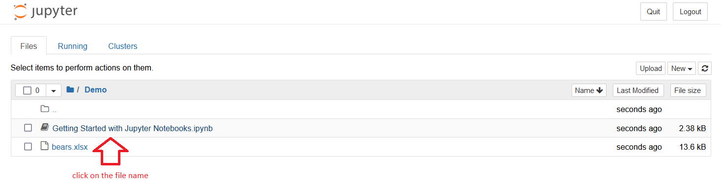
(i) the Jupyter Notebook “Getting Started with Jupyter Notebooks.ipynb”

(ii) the Excel file “bears.xlsx”

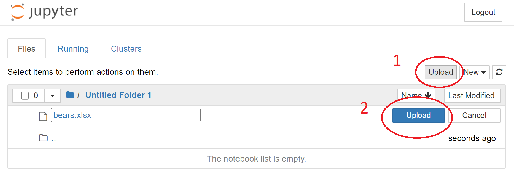
4. Upload the two files in step two into your JNB directory:

5. Open the JNB “Getting Started with Jupyter Notebooks” and follow the instuctions.

2.3.2. Functions

Note

The Python program language is one of the most popular worldwide. It is used widely by data scientists, a profession that is in high demand and well paid if you are good at it. In this demo, we introduce the concept of a function.

1. Here we define a function called add(a,b) that computes the sum a+b. Hit shift+enter to execute the next cell which creates our function. The # symbol is followed by a comment about the code

def add(a,b):   #make sure you include the :
    x = a+b   #make sure you indent
    return x  #return is a key word found at the last line of the code defining the function

2. Here is an an example how we can use the function we just created to compute 5+3. (Always hit shift+enter to execute the cell).

add(5,3)

3. Now it’s your turn. Define a function called subtract(a,b) which computes a-b. Then test that your function is working by showing subtract(5,3) is equal to 5-3=2.

#Define your function subtract(a,b) in this cell

def subtract(a,b):
    y = a-b
    return y

#Test your function by computing subtract(5,3) in this cell. (Make sure you pressed shift+enter in the previous cell.)
subtract(4,5)

-1

4. Now read and execute the next cell. Remember # is the start of a comment.

# Let's define a function multiply(a,b) and then test it on multiply(5,3)
def multiply(a,b):
    x=a*b
    return x
multiply(5,3)

5. Now it’s your turn. Define a function divide(a,b) and test it on divide(5,3). Note that the symbol for divide is /

# Define your function divide(a,b) in this cell

def divide(a,b):
    z=a/b
    return z

# Test your function by computing divide(5,3) in this cell
divide(3,6)

0.5

6. CHALLENGE 1: Can you solve the following math problem by providing the correct input to the Python function?

Study the code below average(a,b,c). Then given that a=2, b=5, figure out the correct value of c so that average(a,b,c)=10.

def average(a,b,c):
    ave = (a+b+c)/3
    return ave

a=2
b=5
c=23 #Here's a guess for c.  Edit it so you get the right answer.
average(a,b,c)

10.0

Congratulations if you defined c in such a way as to get 10.0.

Note

Your instructor may ask you to submit a file of your completed work.

You can create a PDF of your completed JNB by selecting File on the top menu bar, and then Print Preview. Right-click, and then print to PDF.

You can also download the JNB itself by selecting File, Download as, Notebook(.ipynb).

Try creating both file formats.

Congratulations! You have succesfully completed this intro to functions!

2.3.3. numpy

Note

In the previous section, we created a few simple functions to get used to how we can create a ‘special work order’ to get the computer to do something for us.

Certain functions are used so often and widely that it really makes no sense for everyone to re-invent the wheel each time by defining a function. Instead, there are ‘libraries’ of functions which can be ‘imported’ for use in our Jupyter Notebook (JNB). We can use any function in an imported library by knowing the name of the function and what inputs are required.

The first library we will use is the ‘numerical Python’ library called ‘numpy’ and abbreviated as ‘np’.

(1) Press shift+enter to execute the next cell which imports the numpy library.

import numpy as np  #this is how we import the numpy library with abbreviated name np

The . extension

(2) We can access a function in the numpy library using

np.

followed by the name of the function.

For example, suppose we wish to create a list of numbers 0,10,20,30,40,50,60,70,80,90,100. There is a numpy library function arange(starting_number,gone_too_far_number,spacing_by) which works well for this task.

In our case, use starting_number=0, gone_too_far_number=110, spacing_by=10.

Remembering to put np. in front of the function, execute the next cell (shift+enter) to see the result.

np.arange(0,110,10)

array([  0,  10,  20,  30,  40,  50,  60,  70,  80,  90, 100])

(3) Now you try it. Use numpy to make a list of all the numbers between 0 and 50.

np.arange(0,51,1)

array([ 0,  1,  2,  3,  4,  5,  6,  7,  8,  9, 10, 11, 12, 13, 14, 15, 16,
       17, 18, 19, 20, 21, 22, 23, 24, 25, 26, 27, 28, 29, 30, 31, 32, 33,
       34, 35, 36, 37, 38, 39, 40, 41, 42, 43, 44, 45, 46, 47, 48, 49, 50])

(4) Inside of a library there might be sub-libraries, akin to a children’s library within a main library. One of numpy’s sub-libraries is called random.

SINGLE CHOICE POP QUIZ How do we access the random library within the numpy library?
a) np.random

If you answered a) np.random you are correct!

Inside the random library is a function called randint(numbers_in_a_hat).

The input value for numbers_in_a_hat is a positive integer like 10. This specifies that ten numbers starting with 0 (i.e. 0,1,2,…,9) will put into a hat.

The function randint(10) then tells the computer to pulls out randomly one of the numbers in our hat.

Remembering to put np.random. in front of the function, try it by hitting shift+enter sveral times in succession on the cell below to simulate random draws from a hat (with replacement).

np.random.randint(10)

1

(5) Now it’s your turn. Tell the computer to pick a random number from a hat which has the numbers 0,2,3,…,999. Do it 3 times to see if you get the same number each time.

#First Try
np.random.randint(1000)

316

#Second Try
np.random.randint(1000)

673

#Third Try
np.random.randint(1000)

814

Hope you enjoyed this quick look at the numpy library!

2.3.4. pandas

Note

Python’s Data Analysis library is called pandas and usually abbreviated as pd. Pandas is one of the most important tools used by Data Scientists today.

1. Let’s begin by importing the library in the same way that we imported the numpy library in JNB2. (Remember to press shift+enter to execute each cell.)

import pandas as pd

File upload

Get the file bears.xlsx from the folder https://drive.google.com/drive/folders/1cpRptbyjYZSENEtjNNEiV7tBrIz4mONI?usp=sharing

Then put the file in the same directory as this Jupyter notebook. (You can do this by choosing File on the top left of the Jupyter Notebook menu bar, and then selecting Open. Then hit the Upload button on the top right, find bears.xlsx, hit Open and then Upload.) Return to this Notebook when you have completed the upload of the datafile.

2. Now we can use the read_excel() function in the pandas library to read the data into what is called a dataframe. We will name our dataframe bear_info.

bear_info=pd.read_excel("bears.xlsx")  #read in the data
bear_info  #display the data

	Animal	Life_Span_in_Years	Size_in_Feet	Weight_in_Pounds
0	Black	20	6	600
1	Giant Panda	20	5	300
2	Grizzly	25	8	800

We can set the names of the columns using the following command.

bear_info.columns=["Type","Age","Size","Weight"]
bear_info

	Type	Age	Size	Weight
0	Black	20	6	600
1	Giant Panda	20	5	300
2	Grizzly	25	8	800

4. We can display just the first two rows of our dataframe using a command of the form df.head(2) where df is the name of our dataframe.

bear_info.head(2)

	Type	Age	Size	Weight
0	Black	20	6	600
1	Giant Panda	20	5	300

5. The column at the left is called the index. Note that the index values start with 0. We can locate information in the dataframe using a command of the form df.loc[index,column] where df is the name of our dataframe, index is the value of the index, and column is the name of the column inside of quotation marks. Here is an example.

bear_info.loc[1,"Weight"]

300

6. Use .loc() to get the age of a Grizzly bear.

#your answer to 6)
bear_info.loc[2,"Age"]

25

7. Use .loc to get the size of a Black bear.

#your answer to 7)
bear_info.loc[0,"Size"]

6

Exercises

Exercises

1. Create your own data file with some interesting info. Read in the data into a dataframe called df using pd.read_excel().

2. Display the first row of df.

3. Abbreviate the column names.

4. Display the first line of your dataframe with abbreviated column names.

5. Show how to use .loc() to get a particular entry in your dataframe.

2.3.5. matplotlib

Note

Matplotlib was created by John Hunter to help make graphs. Like numpy and pandas, matplotlib is a widely used Python library. Dr. Hunter’s used this library as a neurobiologist, studying epilepsy at the University of Chicago. Unfortunately, Dr. Hunter died of cancer at age 44.

1. The matplotlib library has a sub-library called pyplot (plt). We can access the functions in pyplot by executing the next cell.

import matplotlib.pyplot as plt

2. Here is an example of a simple plot.

# create a new figure
plt.figure()
# plot the points (0, 1) (1,0),(2,1),(3,0) and (4,1) with a 'o' marker and connect them using 'o'
xvalues=[0,1,2,3,4]
yvalues=[1,0,1,0,1]
plt.plot(xvalues, yvalues, 'o-',color='blue')

[<matplotlib.lines.Line2D at 0x1ee01c76490>]

3. Use pyplot to create a red letter M.

#Your answer to 3)
plt.figure()
xvalues=[0,1,2,3,4]
yvalues=[0,1,0,1,0]
plt.plot(xvalues, yvalues, 'o-',color='red')

[<matplotlib.lines.Line2D at 0x1ee0395cb10>]

4. Let’s make a simple bargraph using pyplot.

plt.figure()
xvals = [0,1,2]
heights=[2,4,6]
plt.bar(xvals, heights, width = 0.3,color='black')

<BarContainer object of 3 artists>

5. Create a bar graph with 4 bars at x positions 1,2,3 and 4 and with heights 2,3,1,5.

# Your answer to 5)

6. One more example is a pie chart.

plt.figure(figsize=(5,5)) #you can adjust the figure size
activities=["work","play","eat","sleep"]
hours=[8,3,3,10]
plt.pie(hours,labels=activities,autopct='%1.1f%%')  #percentages are automatically computed

([<matplotlib.patches.Wedge at 0x2cfb95c8f50>,
  <matplotlib.patches.Wedge at 0x2cfb95ca990>,
  <matplotlib.patches.Wedge at 0x2cfb95d0690>,
  <matplotlib.patches.Wedge at 0x2cfb95d21d0>],
 [Text(0.5499999702695115, 0.9526279613277875, 'work'),
  Text(-0.8726887161176864, 0.6696375174382514, 'play'),
  Text(-1.0905893385493104, -0.1435788795142854, 'eat'),
  Text(0.2847009827728232, -1.0625184000327659, 'sleep')],
 [Text(0.2999999837833699, 0.5196152516333385, '33.3%'),
  Text(-0.4760120269732834, 0.36525682769359163, '12.5%'),
  Text(-0.5948669119359874, -0.07831575246233749, '12.5%'),
  Text(0.15529144514881263, -0.5795554909269631, '41.7%')])

7. Make a piechart which describes your usual daily activities and how long you spend on each.

#Your answer to 7)

2.3.6. for loops

Note

In this section, we will introduce a “for loop” as a tool to build more complicated user-defined functions introduced in JNB1. We will also make use of the numpy library function arange(). (It might be good to go back and review the previous sections.)

1. Let’s start by importing the numpy library. (Don’t forget to press shift+enter to execute each cell.)

import numpy as np

2. Let’s create a list of all numbers between 1 and 10.

my_list=np.arange(1,11,1)
my_list

array([ 1,  2,  3,  4,  5,  6,  7,  8,  9, 10])

3. Python has technical names for the things we create. The built-in type() function will give us the technical name. Let’s check the technical name for our list.

type(my_list)

numpy.ndarray

4. Let’s define a function which takes an input list and outputs the square of each number in the list. A for loop is used to go through one by one the numbers in a list.

def squared(my_list):  #remember the use of :
    for i in my_list:  #must indent lines in a function; for loops need a :
        print(i**2)       #must also indent lines in a for loop
    return print("Finished!")  #prints a message to the screen when completed

5. Let’s see if this works.

squared(my_list)

1
4
9
16
25
36
49
64
81
100
Finished!

6. The cube of a number is the number multiplied by itself 3 times. For example, \(2^3=8\) and \(10^3=1000\). In Python we write \(2**3\) and \(10**3\) to get the computer to compute these cubes. Define a function called cube which cubes each number in an input list and then returns the message “That was easy!” Test out your function on the list we defined earlier.

#definition of the function
def cubed(my_list):
    for i in my_list:
        print(i**3)
    return print("That was easy!")

#test of the function
cubed(my_list)

1
8
27
64
125
216
343
512
729
1000
That was easy!

Exercise

Exercise

Define a new list called list1 which has all the even numbers between 0 and 10. Then define a function called addone which adds one to each number in list1 and prints “Mission Accomplished!” when done. Test that your function does what it is supposed to do.

2.3.7. if conditional statements

Note

In this section, we will introduce an if conditional statement as another useful tool in its own right and in writing user-defined functions. Basically a command(s) is executed only if a specified condition is true. If not, there is an ‘else’ option to specify a different command(s) to be executed.

1. Let’s start by importing the numpy library. (Don’t forget to press shift+enter to execute each cell.)

import numpy as np

2. Let’s create a ist of all numbers between 1 and 10.

list=np.arange(1,11,1)
list

array([ 1,  2,  3,  4,  5,  6,  7,  8,  9, 10])

3. Let’s define a function checksize which takes an input list and outputs whether each number in the list is less than 7. If so, the computer will print “OK” and if not, the computer will print “Too Big!”

def checksize(list):  #remember the use of :
    for i in list:  #the for statement needs a : at the end. The next line  must also be indented.
        if i<7:     #an if statement also needs a : at the end;  must also indent the next line
            print(i,"is OK")   # computer does this if i<7
        else:      # else needs a : at the end; must indent the next line
            print(i, "is Too Big!") # instruction if x >=7
    return print("Finished!")  #prints a message to the screen when completed

4. Let’s see if this works.

checksize(list)

1 is OK
2 is OK
3 is OK
4 is OK
5 is OK
6 is OK
7 is Too Big!
8 is Too Big!
9 is Too Big!
10 is Too Big!
Finished!

5. Create a new list called list1 consisting of numbers from 1 to 20. Define a function numberdigits(list1) which goes through the numbers in list1 and prints “is single digit” if the number is single digit and “is double digits” if the number is double digit. Check that your function runs correctly on list1.

#define list 1 
list1=np.arange(1,21,1)

#definition of the function
def numberdigits(list1):
    for i in list1:
        if i<10:
            print(i,"is single digit")
        else:
            print(i,"is double digits")

#test of the function
numberdigits(list1)

1 is single digit
2 is single digit
3 is single digit
4 is single digit
5 is single digit
6 is single digit
7 is single digit
8 is single digit
9 is single digit
10 is double digits
11 is double digits
12 is double digits
13 is double digits
14 is double digits
15 is double digits
16 is double digits
17 is double digits
18 is double digits
19 is double digits
20 is double digits

Exercise

Exercise

Define a new list called list2 which has all the even numbers between 0 and 20. Then define a function halve_upper_half(list2) which outputs half of each number in list2 if the original number is greater than 10. Check that your function does what it is supposed to do.

2.3.8. dataframes

Note

One important use of dataframes is the analysis of real world data. For such analysis, the basic Python skills we have introduced so far are all utilized:

• (user-defined) functions

• the numpy library

• the pandas library

• the matplotlib library

• for loops

• if conditionals

We will use a dataframe called COVID to explore COVID-19 data imported directly from the City of Chicago’s Data Portal.

1. Let’s start by importing the numpy and pandas libraries. In general, we will always begin by importing these two libraries (Don’t forget to press shift+enter to execute each cell.)

import numpy as np
import pandas as pd

2. We can use pandas (pd) to get up-to-date info about COVID 19. Let’s create a dataframe called COVID with this info and display the first line.

COVID=pd.read_json("https://data.cityofchicago.org/resource/yhhz-zm2v.json?$limit=5000000")
COVID.head(1)

	zip_code	week_number	week_start	week_end	cases_weekly	cases_cumulative	case_rate_weekly	case_rate_cumulative	tests_weekly	tests_cumulative	...	death_rate_weekly	death_rate_cumulative	population	row_id	zip_code_location	:@computed_region_rpca_8um6	:@computed_region_vrxf_vc4k	:@computed_region_6mkv_f3dw	:@computed_region_bdys_3d7i	:@computed_region_43wa_7qmu
0	60615	12	2024-03-17T00:00:00.000	2024-03-23T00:00:00.000	4.0	10642.0	9.6	25604.5	0.0	0	...	0.0	194.9	41563	60615-2024-12	{'type': 'Point', 'coordinates': [-87.602725, ...	10.0	8.0	21192.0	147.0	33.0

1 rows × 26 columns

3. Let’s list just the columns in the COVID dataframe.

COVID.columns

Index(['zip_code', 'week_number', 'week_start', 'week_end', 'cases_weekly',
       'cases_cumulative', 'case_rate_weekly', 'case_rate_cumulative',
       'tests_weekly', 'tests_cumulative', 'test_rate_weekly',
       'test_rate_cumulative', 'percent_tested_positive_weekly',
       'percent_tested_positive_cumulative', 'deaths_weekly',
       'deaths_cumulative', 'death_rate_weekly', 'death_rate_cumulative',
       'population', 'row_id', 'zip_code_location',
       ':@computed_region_rpca_8um6', ':@computed_region_vrxf_vc4k',
       ':@computed_region_6mkv_f3dw', ':@computed_region_bdys_3d7i',
       ':@computed_region_43wa_7qmu'],
      dtype='object')

4. Let’s get the number of rows and columns in our dataframe.

COVID.shape

(10560, 26)

5. Let’s use just 4 columns: deaths_cumulative, population, tests_cumulative, and zip_code.

COVID=COVID[["deaths_cumulative", "population", "tests_cumulative","zip_code"]]
COVID.head(1)

	deaths_cumulative	population	tests_cumulative	zip_code
0	2	14675	198	60601

6. Let’s shorten the column names.

COVID.columns=["deaths","population","tests","zip"]
COVID.head(15)

	deaths	population	tests	zip
0	2	14675	198	60601
1	11	14675	23059	60601
2	5	14675	5654	60601
3	12	14675	58296	60601
4	5	14675	782	60601
5	5	14675	1075	60601
6	5	14675	1439	60601
7	6	14675	6044	60601
8	6	14675	6437	60601
9	6	14675	6870	60601
10	7	14675	7642	60601
11	7	14675	8222	60601
12	7	14675	8798	60601
13	7	14675	9377	60601
14	8	14675	10125	60601

7. We can get the latest test info for zip 60601 by first creating a datframe df for that zip code, and then using max() to get the highest value in the “tests” column.

df = COVID[COVID["zip"]=='60601']
numtested=df["tests"].max()
numtested

104307

8. Let’s define a function MyCOVID(COVID,zip) which allows us to enter a 5-digit zip code number and have the computer tell us how many tests, and the number of deaths.

def MyCOVID(COVID,zipcode):
    alreadychecked=0  #eliminate duplication of information
    for z in COVID.index:  #go through all the index values
        if COVID.loc[z,"zip"]==zipcode and alreadychecked==0:    #found the zip we requested (first-time)
            alreadychecked=1  #we will only do this once
            df=COVID[COVID["zip"]==zipcode]
            numtested=df["tests"].max()
            numdeaths=df["deaths"].max()
            print("Zip code: ", COVID.loc[z,"zip"])
            print("number tested is ", numtested)
            print("number deaths ", numdeaths)
    return ("Enter a different zip code if you wish.")

9. Let’s see if there’s data for zipcode=‘60623’.

zipcode='60623'
MyCOVID(COVID,zipcode)

Zip code:  60623
number tested is  436762
number deaths  334

'Enter a different zip code if you wish.'

10. Now analyze zipicode=‘60637’

zipcode=‘60637’ MyCOVID(COVID,zipcode)

Exercise

Exercise

Modify the MyCOVID function so that a function MyCOVID2 also includes the population of the input zipcode. Then check that your function works on zipcode=‘60637’