Orthogonality

9.6. Orthogonality#

import numpy as np
from matplotlib import pyplot as plt

9.6.1. Inner Products and Orthogonality#

In this section, we explore inner products and orthogonality. Inner products allow us to define intuitive geometric concepts such as length, distance, and perpendicularity in $n$ dimensional space $R^{n}$ .

Inner product#

Let $\vec{u}$ and $\vec{v}$ be vectors in $R^{n}$ . We can view them as $n \times 1$ matrices. The transpose of $\vec{u}$ , denoted as ${\vec{u}}^{T}$ , is a $1 \times n$ matrix. The matrix product of ${\vec{u}}^{T}$ and $\vec{v}$ yields a $1 \times 1$ matrix, which can be written as a real number (a scalar) without brackets. This scalar is known as the inner product or dot product of $\vec{u}$ and $\vec{v}$ . To compute it, we multiply the corresponding elements of $\vec{u}$ and $\vec{v}$ and sum the results. More precisely, if

\begin{array}{r} \vec{u} = [\begin{array}{c} u_{1} \\ u_{2} \\ ⋮ \\ u_{n} \end{array}] \end{array}

and

\begin{array}{r} \vec{v} = [\begin{array}{c} v_{1} \\ v_{2} \\ ⋮ \\ v_{n} \end{array}], \end{array}

then the dot product $\vec{u} \cdot \vec{v}$ is given by:

\begin{array}{r} \vec{u} \cdot \vec{v} = {\vec{u}}^{T} \vec{v} = [\begin{array}{c} u_{1} & u_{2} & \dots & u_{n} \end{array}] [\begin{array}{c} v_{1} \\ v_{2} \\ ⋮ \\ v_{n} \end{array}] = u_{1} v_{1} + u_{2} v_{2} + \dots + u_{n} v_{n} \end{array}

Example 1

Compute $\vec{u} \cdot \vec{v}$ for $\vec{u} = [\begin{matrix} 1 \\ - 1 \\ 2 \end{matrix}]$ and $\vec{v} = [\begin{matrix} - 2 \\ 3 \\ 4 \end{matrix}]$ .

Solution

We use numpy.dot() to compute the dot product in Python:

import numpy as np

u = np.array([1, -1, 2])
v = np.array([-2, 3, 4])

uv = np.dot(u,v)
uv

Theorem 1 (Properties of the dot product)

Let $\vec{u}$ , $\vec{v}$ and $\vec{w}$ be vectors in $R^{n}$ , and $c \in R$ be a scalar. Then

$\vec{u} \cdot \vec{v} = \vec{v} \cdot \vec{u} .$
$(\vec{u} + \vec{v}) \cdot \vec{w} = \vec{u} \cdot \vec{w} + \vec{v} \cdot \vec{w} .$
$c (\vec{u} \cdot \vec{v}) = (c \vec{u}) \cdot \vec{v} = \vec{u} \cdot (c \vec{v}) .$
$\vec{u} \cdot \vec{v} \geq 0$ , and $\vec{u} \cdot \vec{u} = 0$ if and only if $\vec{u} = 0.$

combining (2) and (3), and using induction we can show:

(c_{1} \vec{u_{1}} + c_{2} {\vec{u}}_{2} \dots c_{p} {\vec{u}}_{p}) \cdot \vec{w} = c_{1} \vec{w} \cdot {\vec{u}}_{1} + c_{2} \vec{w} \cdot {\vec{u}}_{2} + \dots c_{p} \vec{w} \cdot {\vec{u}}_{p}

Length of vectors

The dot product can be used to define the length of vectors: let $\vec{u} \in R^{n}$ then the magnitude or the length of $\vec{u}$ , denoted by $‖ \vec{u} ‖$ is defined by

‖ \vec{u} ‖ = \sqrt{\vec{u} \cdot \vec{u}} .

Note that this definition of length coincides with the standard notion of length in $R^{2}$ and $R^{3}$ .
A vector with a length of $1$ is called a unit vector. For any vector $\vec{u}$ , there exists a unit vector in the direction of $\vec{u}$ . To obtain this vector, we first calculate the length of $\vec{u}$ and then divide $\vec{u}$ by its length $‖ \vec{u} ‖$ . The resulting vector is referred to as the unit vector of $\vec{u}$ , and commonly denoted as ${\vec{e}}_{u}$ :

{\vec{e}}_{u} = \frac{\vec{u}}{‖ \vec{u} ‖}

This process is often called normalizing a vector, as it transforms $\vec{u}$ into a unit vector by scaling it to have a length of $1$ .

Example 2

Let $\vec{u} = [\begin{matrix} 1 \\ 2 \\ 3 \end{matrix}]$ . Compute the following:

$‖ \vec{u} ‖$
$‖ - 2 \vec{u} ‖$
${\vec{e}}_{u}$

Solution:

# (1)

u = np.array([1,2,3])

uu = np.dot(u,u)

length_u = np.sqrt(uu)

length_u

3.7416573867739413

# (2)

v = -2*u

vv = np.dot(v,v)

length_v = np.sqrt(vv)

length_v

7.483314773547883

We could also use the properties of the dot products to compute $‖ - 2 \vec{u} ‖$ :

‖ - 2 \vec{u} ‖ = \sqrt{- 2 \vec{u} \cdot - 2 \vec{u}} = 2 (\vec{u} \cdot \vec{u}) = 2 ‖ \vec{u} ‖

#(3) computing the unit vector of u

e_u = u/length_u

e_u

array([0.26726124, 0.53452248, 0.80178373])

Let’s check that the length of ${\vec{e}}_{u}$ is exactly 1:

length_e = np.sqrt(np.dot(e_u,e_u))

length_e

1.0

Example 3

Given vectors

\begin{array}{r} \vec{u} = [\begin{array}{c} 1 \\ - 1 \\ 2 \end{array}] \end{array}

and

\begin{array}{r} \vec{v} = [\begin{array}{c} - 2 \\ 3 \\ 4 \end{array}], \end{array}

and the subspace $W$ spanned by $\vec{u}$ and $\vec{v}$ , find unit vectors ${\vec{w}}_{1}$ and ${\vec{w}}_{2}$ that form a basis for $W$ .

Solution:

Since $\vec{u}$ and $\vec{v}$ are linearly independent (they are not scalar multiples of each other), we can proceed to normalize them to get unit vectors.

# unit vector of u
u = np.array([1,-1,2])
e_u = u / np.sqrt(np.dot(u,u))


# unit vector of v
v = np.array([-2, 3, 4])
e_v = v / np.sqrt(np.dot(v,v))


print("e_u = ", e_u)
print("e_v = ", e_v)

e_u =  [ 0.40824829 -0.40824829  0.81649658]
e_v =  [-0.37139068  0.55708601  0.74278135]

Distance in $R^{n}$

For $\vec{u}$ and $\vec{v}$ in $R^{n}$ , the distance between $\vec{u}$ and $\vec{v}$ , denoted by $dist (\vec{v}, \vec{u})$ , is the length of their difference vector $\vec{u} - \vec{v}$ . That is,

dist (\vec{u}, \vec{v}) = ‖ \vec{u} - \vec{v} ‖ .

Note that this definition coincides with the standard definition of distances in $R^{2}$ and $R^{3}$ .

Example 4

Compute the distance between vectors in Example 2.

Solution:

w = u - v

dist = np.sqrt(np.dot(w,w))

print("The distance between ", u, " and ", v, " is ", dist)

The distance between  [1 2 3]  and  [-2 -4 -6]  is  11.224972160321824

Angles and Orthogonality#

Theorem 2 (Cauchy-Schwarz inequality)

For $\vec{u}$ and $\vec{v}$ in $R^{n}$ we have

| \vec{u} \cdot \vec{v} | \leq ‖ \vec{u} ‖ ‖ \vec{v} ‖ .

The Cauchy-Schwarz inequality gives us a way to define the notion of an angle between two $n$ dimensional vectors $\vec{u}$ and $\vec{v}$ . This notion also coincides with our intuition in $R^{2}$ and $R^{3}$ :

Suppose $\vec{u}, \vec{v} \in R^{n}$ are non-zero vectors. Note that

- 1 \leq \frac{\vec{u} \cdot \vec{v}}{‖ \vec{u} ‖ ‖ \vec{v} ‖} \leq 1

Therefore, there is a unique $θ \in [0, π]$ such that

\cos (θ) = \frac{\vec{u} \cdot \vec{v}}{‖ \vec{u} ‖ ‖ \vec{v} ‖}

$θ$ is referred to as the angle between $\vec{u}$ and $\vec{v}$ and is equal to

θ = \arccos (\frac{\vec{u} \cdot \vec{v}}{‖ \vec{u} ‖ ‖ \vec{v} ‖})

Example 5

Find the angle between vectors in Example 2.

Solution:

We first compute the length of $\vec{u}$ and $\vec{v}$ and then substitute them in above formula:

u_len = np.sqrt(np.dot(u,u))
v_len = np.sqrt(np.dot(v,v))

z = u_len * v_len

t = np.arccos(np.dot(u,v)/z)       
print("The angle between u and v is ", t ," rad")

---------------------------------------------------------------------------
NameError                                 Traceback (most recent call last)
Cell In[6], line 1
----> 1 u_len = np.sqrt(np.dot(u,u))
      2 v_len = np.sqrt(np.dot(v,v))
      4 z = u_len * v_len

NameError: name 'u' is not defined

Two vectors $\vec{u}$ and $\vec{v}$ are orthogonal, denoted by $\vec{u} ⊥ \vec{v}$ , if the angle $θ$ between them is $\frac{π}{2}$ . Alternatively, this condition is satisfied if and only if $\vec{u} \cdot \vec{v} = 0$ . It is worth noting that the zero vector $\vec{0}$ is orthogonal to every vector because ${\vec{0}}^{T} \cdot \vec{u} = 0$ for any vector $\vec{u}$ .

Observe that for any two vectors $\vec{u}$ and $\vec{v}$ we have

‖ \vec{u} + \vec{v} ‖^{2} = (\vec{u} + \vec{v}) \cdot (\vec{u} + \vec{v}) = ‖ \vec{u} ‖^{2} + ‖ \vec{v} ‖^{2} + 2 \vec{u} \cdot \vec{v} .

The above calculation implies the famous Pythagorean Theorem:

Theorem 3 (The Pythagorean Theorem)

Two vectors $\vec{u}$ and $\vec{v}$ are orthogonal if and only if

‖ \vec{u} + \vec{v} ‖^{2} = ‖ \vec{u} ‖^{2} + ‖ \vec{v} ‖^{2}

The orthogonal complement of a subspace

Let $W \subset R^{n}$ be a subspace. If a vector $\vec{u}$ is orthogonal to every vector in the subspace $W$ , then $\vec{u}$ is said to be orthogonal to $W$ . The set of all vectors $\vec{u}$ that are orthogonal to $W$ form a subspace which is commonly called the orthogonal complement of $W$ and is denoted by $W^{⊥}$ (or simply $W^{⊥}$ ):

W^{⊥} = {\vec{u} \in R^{n} : \vec{u} \cdot \vec{w} = 0 for all \vec{w} \in W}

Example 6

Let $W$ be the $x y$ -plane in $R^{3}$ , and let $L$ be the $z$ -axis. Our intuition says $L$ is orthogonal to $W$ . In fact, if $\vec{z}$ and $\vec{w}$ are nonzero vectors such that $\vec{z} \in L$ and $\vec{w} \in W$ , then $\vec{z}$ is orthogonal to $\vec{w}$ . Since $\vec{w}$ and $\vec{z}$ were chosen arbitrarily, every vector on $L$ is orthogonal to every $\vec{w}$ in $W$ . In fact, $L$ consists of all vectors that are orthogonal to the $\vec{w}$ ’s in $W$ , and $W$ consists of all vectors $\vec{w}$ orthogonal to the $\vec{z}$ ’s in $L$ . Mathematically,

L = W^{⊥} and W = L^{⊥}

Example 7

If $W = s p a n {[\begin{matrix} 1 \\ 0 \\ 0 \end{matrix}]}$ , find a basis for $W^{⊥}$ .

Solution:

Note that $W$ is simply the $x$ -axis in $R^{3}$ . Intuitively, $W^{⊥}$ should be the $y z$ -plane, and a basis for it is

\begin{array}{r} B = {[\begin{array}{c} 0 \\ 1 \\ 0 \end{array}], [\begin{array}{c} 0 \\ 0 \\ 1 \end{array}]} . \end{array}

Alternatively, we can find the solutions to the linear system:

\begin{array}{r} [\begin{array}{c} 1 & 0 & 0 \end{array}] [\begin{array}{c} x \\ y \\ z \end{array}] = \vec{0} . \end{array}

We have:

\begin{array}{r} [\begin{array}{c} x \\ y \\ z \end{array}] = [\begin{array}{c} 0 \\ y \\ z \end{array}] = y [\begin{array}{c} 0 \\ 1 \\ 0 \end{array}] + z [\begin{array}{c} 0 \\ 0 \\ 1 \end{array}] . \end{array}

We conclude this section with a theorem summarizing the properties of the orthogonal complement of a subspace.

Theorem 4

Let $W$ be a subspace of $R^{n}$ .

The orthogonal complement $W^{⊥}$ is also a subspace of $R^{n}$ .
The sum of the dimensions of $W$ and $W^{⊥}$ is equal to the dimension of the ambient space $R^{n}$ , i.e., $d i m (W) + d i m (W^{⊥}) = n$ .
If $W$ is the column space of some matrix $A$ , i.e., $W = col (A)$ , then $W^{⊥}$ is precisely the null space of the transpose of $A$ , i.e., $W^{⊥} = null (A^{T})$ .

Exercises#

Exercises

Let $\vec{a} = [\begin{matrix} 1 \\ 2 \\ 3 \\ 4 \end{matrix}]$ .

a. Find a vector $\vec{w}$ that is in the opposite direction of $\vec{a}$ and has a magnitude of 2.

b. Find two non-parallel vectors $\vec{u}$ and $\vec{v}$ which are both orthogonal to $\vec{a}$
Find two non-parallel vectors $\vec{u}$ and $\vec{v}$ which are both orthogonal to $[\begin{matrix} 1 \\ 2 \\ 3 \end{matrix}]$ and $[\begin{matrix} 2 \\ - 1 \\ 0 \end{matrix}] .$
Let

\begin{array}{r} \vec{v} = [\begin{array}{c} 1 \\ 2 \\ 7 \end{array}] \end{array}

and

\begin{array}{r} \vec{w} = [\begin{array}{c} 1 \\ - 1 \\ 1 \end{array}] . \end{array}

a. Find $\vec{z} = \vec{v} - (\frac{\vec{v} \cdot \vec{w}}{\vec{w} \cdot \vec{w}}) \vec{w} .$

b. Check that $\vec{z}$ is orthogonal to $\vec{w} .$

If

\begin{array}{r} W = s p a n {[\begin{array}{c} 1 \\ 2 \\ 3 \\ 4 \end{array}]} \end{array}

find a basis for $W^{⊥}$ .

9.6.2. Orthogonal Projection#

In this section, we explore the construction of orthogonal projections, which is a key step in many calculations involving orthogonality, and properties of projection maps.

Orthogonal Set#

A set of vectors ${{\vec{u}}_{1}, {\vec{u}}_{2}, \dots, {\vec{u}}_{p}}$ in $R^{n}$ is called an orthogonal set if each pair of distinct vectors from the set is orthogonal, meaning that ${\vec{u}}_{i} \cdot {\vec{u}}_{j} = 0$ whenever $i \neq j$ . It is important to note that an orthogonal set, consisting of nonzero vectors, is always a linearly independent set. For that reason, if a basis for a subspace $W$ of $R^{n}$ happens to be an orthogonal set, it is called an orthogonal basis.

In general, an orthogonal basis makes computations easier. The following theorem demonstrates how:

Theorem 5

Let

B = {{\vec{u}}_{1}, {\vec{u}}_{2}, \dots, {\vec{u}}_{p}}

be an orthogonal basis for a subspace $W \subset R^{n}$ . Moreover, suppose $y \in W$ can be expressed as a linear combination of the basis elements:

\vec{y} = c_{1} {\vec{u}}_{1} + c_{2} {\vec{u}}_{2} + \dots + c_{p} {\vec{u}}_{p} .

Then the weights $c_{i}$ are given by

c_{i} = \frac{{\vec{u}}_{i} \cdot \vec{y}}{{\vec{u}}_{i} \cdot {\vec{u}}_{i}} \forall i \in {1, 2, \dots, p} .

Example 1

Write the vector

\begin{array}{r} \vec{y} = [\begin{array}{c} 6 \\ 1 \\ - 8 \end{array}] \end{array}

as a linear combination of the vectors in

\begin{array}{r} S = {[\begin{array}{c} 3 \\ 1 \\ 1 \end{array}], [\begin{array}{c} - 1 \\ 2 \\ 1 \end{array}], [\begin{array}{c} - 1 \\ - 4 \\ 7 \end{array}]} . \end{array}

Solution:

Since $S$ is an orthogonal set with three nonzero elements, it forms a basis for $R^{3}$ . Therefore, we can express $\vec{y}$ in terms of the vectors in $S$ :

\begin{array}{r} \vec{y} = c_{1} [\begin{array}{c} 3 \\ 1 \\ 1 \end{array}] + c_{2} [\begin{array}{c} - 1 \\ 2 \\ 1 \end{array}] + c_{3} [\begin{array}{c} - 1 \\ - 4 \\ 7 \end{array}] . \end{array}

We can solve this vector equation for $c_{i}$ s using techniques we learned in section 1.2. However, Theorem 1 suggests an alternative way of computing the coefficients:

c_{i} = \frac{{\vec{u}}_{i} \cdot \vec{y}}{{\vec{u}}_{i} \cdot {\vec{u}}_{i}} for all i \in {1, 2, 3} .

By substituting the appropriate values of ${\vec{u}}_{i}$ and $\vec{y}$ into the formula, we can compute the coefficients $c_{i}$ s.

y = np.array([6, 1, -8])

u1 = np.array([3, 1, 1])

u2 = np.array([-1, 2, 1])

u3 = np.array([-1,-4, 7])

#computing the weights:

c1 = np.dot(y,u1)/ np.dot(u1,u1)

c2 = np.dot(y,u2)/ np.dot(u2,u2)

c3 = np.dot(y,u3)/ np.dot(u3,u3)

print("c1 = ", c1, ", c2 = ", c1, ", c3 = ", c3)

c1 =  1.0 , c2 =  1.0 , c3 =  -1.0

Orthogonal Projections onto $1$ -dimensional spaces#

Given a nonzero vector $\vec{y}$ in $R^{n}$ , decomposing $\vec{y}$ into a sum of two vectors is a straightforward task. For example, for any choice of $α, β \in R$ such that $α + β = 1$ , we have:

\vec{y} = α \vec{y} + β \vec{y} .

A more challenging question is when we want to express $\vec{y}$ as the sum of two vectors, where one is a scalar multiple of a given vector $\vec{u}$ and the other is orthogonal to $\vec{u}$ . More specifically, we seek to write:

\vec{y} = \vec{p} + \vec{z},

where $\vec{p} = α \vec{u}$ for some scalar $α$ , and $\vec{z} ⊥ \vec{p}$ . In other words, we are looking for a scalar $α$ such that $\vec{z} := \vec{y} - α \vec{u}$ is orthogonal to $\vec{u}$ , which can be expressed as:

(\vec{y} - α \vec{u}) \cdot \vec{u} = 0.

Simplifying the equation above, we find:

α = \frac{\vec{y} \cdot \vec{u}}{\vec{u} \cdot \vec{u}}, and thus \vec{p} = \frac{\vec{y} \cdot \vec{u}}{\vec{u} \cdot \vec{u}} \vec{u}, and \vec{z} = \vec{y} - \vec{p} .

The vector $\vec{p}$ , sometimes denoted as ${proj}_{\vec{u}} (\vec{y})$ , is called the orthogonal projection of $\vec{y}$ onto $\vec{u}$ , and $\vec{z}$ is referred to as the component of $\vec{y}$ orthogonal to $\vec{u}$ .

Example 2

Suppose

$\vec{y} = [\begin{matrix} 7 \\ 6 \end{matrix}]$ and $\vec{u} = [\begin{matrix} 4 \\ 2 \end{matrix}] .$

Compute the ${proj}_{\vec{u}} (\vec{y})$ and the component of $\vec{y}$ orthogonal to $\vec{u}$

Solution:

# setup vectors

y = np.array([7,6])

u = np.array([4,2])

# projection of y onto u

proj_y_u = (np.dot(y,u)/ np.dot(u,u))* u
print( "the projection of y onto u is ", proj_y_u) 

z = y - proj_y_u

print("the component of y orthogonal to u is", z )

the projection of y onto u is  [8. 4.]
the component of y orthogonal to u is [-1.  2.]

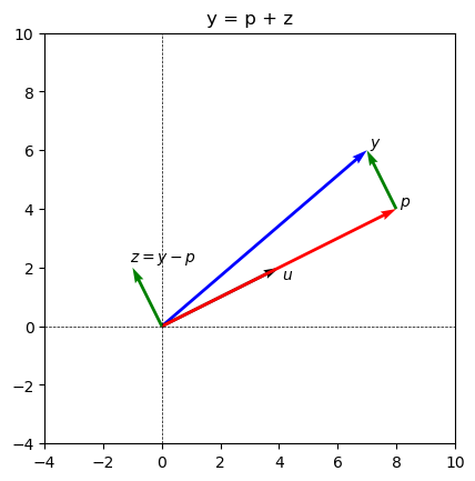
Let’s plot ${proj}_{\vec{u}} (\vec{y})$ and the component of $\vec{y}$ orthogonal to $\vec{u}$ in $x y$ -plane:

# Plot the coordinates in two separate plots
fig, ax = plt.subplots()

figsize=(20, 10)

# vector y
ax.quiver(0, 0, 7, 6, angles='xy', scale_units='xy', scale=1, color='blue', label ='y')
ax.text(7.1,6.1,'$y$')

# vector u
ax.quiver(0, 0, 4, 2, angles='xy', scale_units='xy', scale=1, color='black')
ax.text(4.1,1.6,'$u$')

# orthogonal projection p
ax.quiver(0, 0, 8, 4, angles='xy', scale_units='xy', scale=1, color='red')
ax.text(8.1,4.1,'$p$')

# vector z
ax.quiver(0, 0, -1, 2, angles='xy', scale_units='xy', scale=1, color='green')
ax.text(-1.1,2.2,'$z = y - p$')

# A copy of vector z starting at the end of vector p
ax.quiver(8, 4, -1, 2, angles='xy', scale_units='xy', scale=1, color='green')



ax.set_xlim([-4, 10])
ax.set_ylim([-4, 10])
ax.set_aspect('equal')
ax.axhline(y=0, color='black', linestyle='--', linewidth=0.5)
ax.axvline(x=0, color='black', linestyle='--', linewidth=0.5)

ax.set_title('y = p + z')


plt.show()

../../_images/aa2fa491c123788abb7f99edf507c333ccd23fce7e069b00448f220de3a5d7d7.png

Orthogonal Projections onto a general subspace#

Let’s take another look at the above Figure from Example 2. The projection of $\vec{y}$ onto any vector in the direction of $\vec{u}$ , results in the same vector ${proj}_{\vec{u}} (\vec{y})$ . In fact, what matters to us is the line that contains $\vec{u}$ (span $({\vec{u}})$ ). With this in mind, we can interpret ${proj}_{\vec{u}} (\vec{y})$ as the projection of $\vec{y}$ onto a subspace of $R^{n}$ generated by $\vec{u}$ , and we can write it as ${proj}_{span (L)} (\vec{y})$ . In fact, the notion of projection can be generalized to any subspace of $R^{n}$ .

Theorem 6

Let $W$ be a subspace of $R^{n}$ . Then each $\vec{y} \in R^{n}$ can be written uniquely as

\vec{y} = \vec{p} + \vec{z}

where $\vec{p}$ is in $W$ and $\vec{z}$ is in $W^{⊥}$ . Moreover, if $B = {{\vec{u}}_{1}, {\vec{u}}_{2}, \dots {\vec{u}}_{p}}$ is any orthogonal basis of $W$ , then

\vec{p} = \frac{\vec{y} \cdot {\vec{u}}_{1}}{{\vec{u}}_{1} \cdot {\vec{u}}_{1}} + \frac{\vec{y} \cdot {\vec{u}}_{2}}{{\vec{u}}_{2} \cdot {\vec{u}}_{2}} + \dots + \frac{\vec{y} \cdot {\vec{u}}_{p}}{{\vec{u}}_{p} \cdot {\vec{u}}_{p}} (* *) and \vec{z} = \vec{y} - \vec{p}

The vector $\vec{p}$ , sometimes denoted by ${proj}_{W} (\vec{y})$ is called the orthogonal projection of $\vec{y}$ onto $W$ , and $\vec{z}$ is called the component of $\vec{y}$ orthogonal to $W$ .

Example 3

Suppose

\begin{array}{r} {\vec{u}}_{1} = [\begin{array}{c} 2 \\ 5 \\ - 1 \end{array}], \end{array}

\begin{array}{r} {\vec{u}}_{2} = [\begin{array}{c} - 2 \\ 1 \\ 1 \end{array}], \end{array}

$W = span ({\vec{u}}_{1}, {\vec{u}}_{2})$ and

\begin{array}{r} \vec{y} = [\begin{array}{c} 1 \\ 2 \\ 3 \end{array}] . \end{array}

Compute the ${proj}_{W} (\vec{y})$ and the component of $\vec{y}$ orthogonal to $\vec{u} .$

Solution:

${\vec{u}}_{1}$ and ${\vec{u}}_{2}$ are orthogonal and form a basis for $W$ ; thus, we can use Theorem 3 to compute the projection of $\vec{y}$ onto $W$ :

# setup vectors

u1 = np.array([2,5,-1])

u2 = np.array([-2,1,1])

y = np.array([1,2,3])

# projection of y onto W

proj_y_W = (np.dot(y,u1)/ np.dot(u1,u1))* u1  +  (np.dot(y,u2)/ np.dot(u2,u2))* u2

print( "The projection of y onto W is ", proj_y_W, '\n') 

# component of y orthogonal to p
z = y - proj_y_W

print("The component of y orthogonal to u is", z )

The projection of y onto W is  [-0.4  2.   0.2] 

The component of y orthogonal to u is [1.4 0.  2.8]

Note that if $\vec{y}$ happens to be in $W$ then ${proj}_{W} (\vec{y}) = \vec{y}$ . We can verify this fact for ${\vec{u}}_{1}$ which we know belongs to $W$ :

proj_u_W = (np.dot(u1,u1)/ np.dot(u1,u1))* u1  +  (np.dot(u1,u2)/ np.dot(u2,u2))* u2
print(proj_u_W)

[ 2.  5. -1.]

The Best Approximation Theorem#

Projections can be viewed as linear transformations:

Consider a subspace $W$ of $R^{n}$ , and let $T_{W} : R^{n} \to W$ be the mapping that sends a vector $\vec{y}$ to its orthogonal projection ${proj}_{W} (\vec{y})$ . It is known that $T_{W}$ is a linear transformation. If $P$ represents the matrix of $T_{W}$ , then $P^{2} = P$ . More precisely,

P \vec{w} \in W \forall \vec{w} \in W

Informally, we say $P$ does not move elements of $W$ . The following theorem states that if $\vec{u}$ is not in $W$ , then $P$ sends it to the closest point in $W$ from $\vec{u}$ .

Theorem 7 (The Best Approximation Theorem)

Let $W$ be a subspace of $R^{2}$ , and let $\vec{y} \in R^{n}$ . The projection of $\vec{y}$ onto $W$ , denoted as $\vec{p} = {proj}_{W} (\vec{y})$ , is the closest point in $W$ to $\vec{y}$ in the following sense:

‖ \vec{y} - \vec{p} ‖ \leq ‖ \vec{y} - \vec{w} ‖ \forall \vec{w} \in W

In particular, if $\vec{y} \in W$ , then the closest point is exactly $\vec{y}$ . We refer to $\vec{p}$ as the best approximation to $\vec{y}$ by elements of $W$ . The real number $‖ \vec{y} - \vec{p} ‖$ ) is interpreted as the distance between the vector $\vec{y}$ and the subspace $W$ .

Example 4

Suppose

\begin{array}{r} {\vec{u}}_{1} = [\begin{array}{c} 5 \\ - 2 \\ 1 \end{array}], \end{array}

\begin{array}{r} {\vec{u}}_{2} = [\begin{array}{c} 1 \\ 2 \\ - 1 \end{array}], \end{array}

$W = span ({\vec{u}}_{1}, {\vec{u}}_{2})$

and

\begin{array}{r} \vec{y} = [\begin{array}{c} - 1 \\ - 5 \\ 10 \end{array}] . \end{array}

What is the closest point to $\vec{y}$ in $W$ ?
Find the distance between $\vec{y}$ and $W$ .

Solution

The closest point is the projection of $\vec{y}$ onto $W$ :

# setup vectors

y = np.array([-1, -5, 10])

u1 = np.array([5, -2, 1])

u2 = np.array([1 , 2, -1])

# projection of y onto W

p = (np.dot(y,u1)/ np.dot(u1,u1))* u1  +  (np.dot(y,u2)/ np.dot(u2,u2))* u2

print( "The projection of y onto W is ", p, '\n') 

# component of y orthogonal to p
z = y - p

print("The component of y orthogonal to u is", z, '\n' )

# distance between y and W
r = np.sqrt(np.dot(z,z))
print("The distance between y and W is", r )

---------------------------------------------------------------------------
NameError                                 Traceback (most recent call last)
Cell In[9], line 3
      1 # setup vectors
----> 3 y = np.array([-1, -5, 10])
      5 u1 = np.array([5, -2, 1])
      7 u2 = np.array([1 , 2, -1])

NameError: name 'np' is not defined

It is possible to simplify the $(* *)$ formula in Theorem 6 which computes projection. First, we need the following definition:

A basis $B$ for a subspace $W$ is called an orthonormal basis if $B$ is an orthogonal basis and every element of $B$ is a unit vector. Any orthogonal basis can be turned into an orthonormal basis by normalizing every basis element.

Theorem 8

Let $W$ be a subspace of $R^{n}$ and $B = {{\vec{u}}_{1}, {\vec{u}}_{2}, \dots {\vec{u}}_{p}}$ be an orthonormal basis of $W$ . Then, for every $\vec{y} \in R^{n}$ , the projection of $\vec{y}$ onto $W$ is

{proj}_{W} (\vec{y}) = \vec{y} \cdot \vec{u_{1}} + \vec{y} \cdot \vec{u_{2}} + \dots + \vec{y} \cdot \vec{u_{p}}

We can also represent this formula even in a more compact form:

if $U = [{\vec{u}}_{1}, \vec{u_{2}}, \dots, {\vec{u}}_{p}]$ then

{proj}_{W} (\vec{y}) = U U^{T} \vec{y} (*)

A matrix whose columns are orthonormal, such as $U$ , is called an orthogonal matrix. For an $n \times n$ orthogonal matrix $U$ , besides (*), we have

U^{T} U = I_{n}

Exercises#

Exercises

Let

\begin{array}{r} B = {[\begin{array}{c} 1 \\ 1 \end{array}], [\begin{array}{c} 1 \\ - 1 \end{array}]} \end{array}

be a basis of $R^{2} .$

a. Check that this is an orthogonal basis.

b. Find the coordinates of the vector

\begin{array}{r} [\begin{array}{c} 3 \\ 5 \end{array}] \end{array}

with respect to the basis $B$

Suppose

\begin{array}{r} {\vec{u}}_{1} = [\begin{array}{c} - 7 \\ 1 \\ 4 \end{array}], \end{array}

\begin{array}{r} {\vec{u}}_{2} = [\begin{array}{c} - 1 \\ 1 \\ - 2 \end{array}], \end{array}

$W = span ({\vec{u}}_{1}, {\vec{u}}_{2})$ and

\begin{array}{r} \vec{y} = [\begin{array}{c} - 9 \\ 1 \\ 6 \end{array}] . \end{array}

a. Show that ${\vec{u}}_{1}$ and ${\vec{u}}_{2}$ are orthogonal.

b. What are the closest points to $\vec{y}$ in $W$ ?

c. Find the distance between $W$ and $\vec{y}$ .

d. Convert ${{\vec{u}}_{1}, {\vec{u}}_{2}}$ into an orthonormal basis for $W$ .

e. Compute the projection of $\vec{y}$ onto $W$ using the $(*)$ formula given in Theorem 4.

f. Write $\vec{y}$ as a sum of two vectors one in $W$ and the other in $W^{⊥}$ .

9.6.3. The Gram–Schmidt Process#

In the previous sections, we saw the importance of working with orthogonal and orthonormal bases. In this section, we explore the Gram–Schmidt process which is a simple algorithm to construct an orthogonal or orthonormal basis from any nonzero subspace of $R^{n}$ .

Idea: construction of an orthogonal basis from a basis with two elements#

To see the idea behind the Gram–Schmidt process let’s review Example 2 in Section 5.2:

Suppose $\vec{y} = [\begin{matrix} 7 \\ 6 \end{matrix}]$ and $\vec{u} = [\begin{matrix} 4 \\ 2 \end{matrix}]$ . $\vec{y}$ and $\vec{u}$ are linearly independent and form a basis for $R^{2}$ . Clearly, as shown in below figure, $\vec{y}$ and $\vec{u}$ are not orthogonal, however $\vec{y}$ and $\vec{z}$ (the component of $\vec{y}$ orthogonal to $\vec{u}$ ) form an orthogonal basis for $R^{2}$

# setup vectors

y = np.array([7,6])

u = np.array([4,2])

# projection of y onto u

proj_y_u = (np.dot(y,u)/ np.dot(u,u))* u
print( "The projection of y onto u is ", proj_y_u) 

z = y - proj_y_u

print("The component of y orthogonal to u is", z )


# Plot the coordinates in two separate plots

fig, ax = plt.subplots()

figsize=(10, 5)

# vector y
ax.quiver(0, 0, 7, 6, angles='xy', scale_units='xy', scale=1, color='blue', label ='y')
ax.text(7.1,6.1,'$y$')

# vector u
ax.quiver(0, 0, 4, 2, angles='xy', scale_units='xy', scale=1, color='black')
ax.text(4.1,1.6,'$u$')

# orthogonal projection p
ax.quiver(0, 0, 8, 4, angles='xy', scale_units='xy', scale=1, color='red')
ax.text(8.1,4.1,'$p$')

# vector z
ax.quiver(0, 0, -1, 2, angles='xy', scale_units='xy', scale=1, color='green')
ax.text(-1.1,2.2,'$z = y - p$')

# A copy of vector z starting at the end of vector p
ax.quiver(8, 4, -1, 2, angles='xy', scale_units='xy', scale=1, color='green')



ax.set_xlim([-4, 10])
ax.set_ylim([-4, 10])
ax.set_aspect('equal')
ax.axhline(y=0, color='black', linestyle='--', linewidth=0.5)
ax.axvline(x=0, color='black', linestyle='--', linewidth=0.5)

ax.set_title('y = p + z')


#plt.tight_layout()
plt.show()

The projection of y onto u is  [8. 4.]
The component of y orthogonal to u is [-1.  2.]

Therefore, we have converted a basis for $R^{2}$ into an orthogonal basis for $R^{2}$ .

Construction of an orthogonal basis from a basis with three elements#

Example 1

Let

\begin{array}{r} {\vec{x}}_{1} = [\begin{array}{c} 1 \\ 1 \\ 1 \\ 1 \end{array}], \end{array}

\begin{array}{r} {\vec{x}}_{2} = [\begin{array}{c} 0 \\ 1 \\ 1 \\ 1 \end{array}], \end{array}

\begin{array}{r} {\vec{x}}_{3} = [\begin{array}{c} 0 \\ 0 \\ 1 \\ 1 \end{array}], \end{array}

and

W = span ({{\vec{x}}_{1}, {\vec{x}}_{2}, {\vec{x}}_{3}}) .

Construct an orthogonal basis for $W$ .

Solution:

The set ${{\vec{x}}_{1}, {\vec{x}}_{2}, {\vec{x}}_{3}}$ is a linearly independent and forms a basis for $W$ . We will construct an orthogonal set of vectors ${{\vec{v}}_{1}, {\vec{v}}_{2}, {\vec{v}}_{3}}$ such that $W = span ({{\vec{v}}_{1}, {\vec{v}}_{2}, {\vec{v}}_{3}})$ .

Step 1:

Define ${\vec{v}}_{1} := {\vec{x}}_{1}$ and $W_{1} := span ({\vec{v}}_{1})$ .

Step 2: We seek a vector $\vec{v_{2}}$ orthogonal to $\vec{v_{1}}$ . Project ${\vec{x}}_{2}$ onto $W_{1}$ ; the component of ${\vec{x}}_{2}$ orthogonal to the subspace $W_{1}$ has the desired property:

{\vec{v}}_{2} = {\vec{x}}_{2} - {proj}_{W_{1}}^{{\vec{x}}_{2}} ⟹ \vec{v_{2}} ⊥ \vec{v_{1}}

Now, let $W_{2} = span ({\vec{v}}_{1}, {\vec{v}}_{2})$ .

# setup vectors

x1 = np.array([1,1,1,1])

x2 = np.array([0,1,1,1])

x3 = np.array([0,0,1,1])

v1 = x1
# projection of x2 onto x1

proj_x2_v1 = (np.dot(x2,v1)/ np.dot(v1,v1))* v1
print( "The projection of x2 onto x1 is ", proj_x2_v1, '\n') 

v2 = x2 - proj_x2_v1

print("The component of x1 orthogonal to W1 is", v2 )

The projection of x2 onto x1 is  [0.75 0.75 0.75 0.75] 

The component of x1 orthogonal to W1 is [-0.75  0.25  0.25  0.25]

Step 3:

We can use a similar approach to construct ${\vec{v}}_{3}$ . We find the orthogonal projection of ${\vec{x}}_{3}$ onto $W_{2}$ and define ${\vec{v}}_{3}$ as the component of ${\vec{x}}_{3}$ that is orthogonal to the subspace $W_{2}$ :

{\vec{v}}_{3} = {\vec{x}}_{3} - {proj}_{W_{2}} ({\vec{x}}_{3})

Since both ${\vec{x}}_{3}$ and ${proj}_{W_{2}} ({\vec{x}}_{3})$ are elements of $W$ , ${\vec{v}}_{3}$ is also in $W$ . Moreover, by definition, ${\vec{v}}_{3}$ is orthogonal to both ${\vec{v}}_{1}$ and ${\vec{v}}_{2}$ . Thus, ${{\vec{v}}_{1}, {\vec{v}}_{2}, {\vec{v}}_{3}}$ forms an orthogonal basis for $W$ .

# projection of x3 onto W2

proj_x3_W2 = (np.dot(x3,v1)/ np.dot(v1,v1))* v1  +  (np.dot(x3,v2)/ np.dot(v2,v2))* v2

print( "the projection of x3 onto W2 is ", proj_x3_W2, '\n') 

# component of y orthogonal to p
v3 = x3 - proj_x3_W2

print("the component of x3 orthogonal to W2 is", v3 )

the projection of x3 onto W2 is  [0.         0.66666667 0.66666667 0.66666667] 

the component of x3 orthogonal to W2 is [ 0.         -0.66666667  0.33333333  0.33333333]

Step 4 (Optional)

Normalizing the basis elements $\vec{v_{1}}$ , $\vec{v_{2}}$ , and $\vec{v_{3}}$ , we will get unit vectors $\vec{e_{1}}$ , $\vec{e_{2}}$ , and $\vec{e_{3}}$ respectively. ${\vec{e_{1}}, \vec{e_{2}}, \vec{e_{3}}}$ is an orthonormal basis for $W$ .

# The unit vector of v1
e1 = v1 / np.sqrt(np.dot(v1,v1))

# The unit vector of v1
e2 = v2 / np.sqrt(np.dot(v2,v2))

# The unit vector of v1
e3 = v3 / np.sqrt(np.dot(v3,v3))

print("e1 = ", e1)
print("e2 = ", e2)
print("e3 = ", e3)

e1 =  [0.5 0.5 0.5 0.5]
e2 =  [-0.8660254   0.28867513  0.28867513  0.28867513]
e3 =  [ 0.         -0.81649658  0.40824829  0.40824829]

The Gram_Schmidt Process#

Theorem 8 (the Gram-Schmidt algorithm)

Let $W \subset R^{n}$ be a non-zero subspace, and ${\vec{x_{1}}, \vec{x_{2}}, \dots, \vec{x_{p}}}$ be a basis for $W$ . Define:

(9.2)#

\begin{aligned} \vec{v_{1}} & = \vec{x_{1}} and W_{1} = span (\vec{v_{1}}), \\ \vec{v_{2}} & = \vec{x_{2}} - {proj}_{W_{1}} (\vec{x_{2}}) and W_{2} = span ({\vec{v_{1}}, \vec{v_{2}}}), \\ ⋮ \\ \vec{v_{p}} & = \vec{x_{p}} - {proj}_{W_{p - 1}} (\vec{x_{p}}) and W_{p} = span ({\vec{v_{1}}, \vec{v_{2}}, \dots, \vec{v_{3}}}) . \end{aligned}

Then $W = W_{p}$ , and ${\vec{v_{1}}, \vec{v_{2}}, \dots, \vec{v_{p}}}$ is an orthogonal basis for $W$ . Moreover, if $\vec{e_{1}}, \vec{e_{2}}, \dots, \vec{e_{p}}$ are the unit vectors of $\vec{v_{1}}, \vec{v_{2}}, \dots, \vec{v_{p}}$ respectively, then ${\vec{e_{1}}, \vec{e_{2}}, \dots, \vec{e_{p}}}$ is an orthonormal basis for $W$ .

# setup A
A = np.transpose([x1, x2, x3])

# setup Q
Q = np.transpose([e1, e2, e3])

# Compute R= Q^T*A
R = np.transpose(Q) @ A

array([[2.00000000e+00, 1.50000000e+00, 1.00000000e+00],
       [1.11022302e-16, 8.66025404e-01, 5.77350269e-01],
       [1.11022302e-16, 1.11022302e-16, 8.16496581e-01]])

Note that elements below the diagonal in $R$ are very small and close to zero. In fact, $R$ should be an upper triangular matrix. The reason why Python won’t display the exact decimal numbers we expect is that some decimal fractions cannot be represented exactly as binary fractions. To address this issue, we can set very small elements of $R$ to zero.

eps = 0.000001 
R[np.abs(R) < eps] = 0
R

array([[2.        , 1.5       , 1.        ],
       [0.        , 0.8660254 , 0.57735027],
       [0.        , 0.        , 0.81649658]])

Numerical Note

When the Gram–Schmidt process is run on a computer, round-off error can build up as the vectors $\vec{v_{k}}$ are calculated, one by one. Specifically, for large and unequal values of $k$ and $j$ , the dot products ${\vec{v_{k}}}^{T} \cdot \vec{u_{j}}$ may not be sufficiently close to zero, leading to a loss of orthogonality. This loss of orthogonality can be reduced substantially by rearranging the order of the calculations.

We can also utilize numpy.linalg.qr in Python to compute the QR factorization of a matrix. This function provides an efficient and accurate implementation of the Gram-Schmidt process avoiding unnecessary loss of orthogonality.

Q, R = np.linalg.qr(A)

print('Q = \n', Q, '\n\n')

print('R = \n', R)

Q = 
 [[-0.5         0.8660254   0.        ]
 [-0.5        -0.28867513  0.81649658]
 [-0.5        -0.28867513 -0.40824829]
 [-0.5        -0.28867513 -0.40824829]] 


R = 
 [[-2.         -1.5        -1.        ]
 [ 0.         -0.8660254  -0.57735027]
 [ 0.          0.         -0.81649658]]

Exercises#

Exercises

Let

\begin{array}{r} {\vec{x}}_{1} = [\begin{array}{c} 3 \\ 1 \\ - 1 \\ 3 \end{array}], \end{array}

\begin{array}{r} {\vec{x}}_{2} = [\begin{array}{c} - 5 \\ 1 \\ 5 \\ - 7 \end{array}], \end{array}

\begin{array}{r} {\vec{x}}_{3} = [\begin{array}{c} 1 \\ 1 \\ - 2 \\ 8 \end{array}], \end{array}

and

W = span ({{\vec{x}}_{1}, {\vec{x}}_{2}, {\vec{x}}_{3}}) .

Construct an orthonormal basis for $W$ .

Let $A$ be a matrix whose columns are ${\vec{x}}_{1}$ , ${\vec{x}}_{2}$ , ${\vec{x}}_{3}$ from Exercise 1:

\begin{array}{r} A = [\begin{array}{c} 3 & - 5 & 1 \\ 1 & 1 & 1 \\ - 1 & 5 & - 2 \\ 3 & - 7 & 8 \end{array}] . \end{array}

Find a QR decomposition for $A$ .

Let $A = Q R$ , where $Q$ is an $m \times n$ matrix with orthogonal columns, and $R$ is an $n \times n$ matrix. Show that if the columns of $A$ are linearly dependent, then $R$ cannot be invertible.

9.6.4. Least-Squares Problems#

Linear systems arising in applications are often inconsistent. In such situations, the best one can do is to find a vector ${\vec{x}}^{'}$ that makes $A \vec{x}$ as close as possible to $\vec{b}$ . We think of $A \vec{x}$ as an approximation of $\vec{b}$ . The smaller $‖ \vec{b} - A \vec{x} ‖$ , the better the approximation. Therefore, we are looking for a vector $\hat{y}$ such that $‖ \vec{b} - A \hat{x} ‖$ is as small as possible. Such $\vec{y}$ is called the least square solution of $A \vec{x} = \vec{b}$ . The name is motivated by the fact that $‖ \vec{b} - A \hat{x} ‖$ is the square root of a sum of squares. In this section, we explore this idea further.

Let $A \vec{x} = \vec{b}$ be inconsistent, which implies $\vec{b} \notin col (A)$ . Note that no matter what $\vec{x}$ is, $A \vec{x}$ lies in $col (A)$ . From Section 5.2, we know that the closest point to $\vec{b}$ in $col (A)$ is the projection of $\vec{b}$ onto $col (A)$ (the best approximation problem). Let $\hat{b} = {proj}_{col (A)} (\vec{b})$ . Since $A \vec{x} = \hat{b}$ is consistent, there are $\hat{x}$ such that $A \hat{x} = \hat{b}$ . $\hat{x}$ is a least square solution of $A \vec{x} = \vec{b}$ . Recall that $\vec{b} - \hat{b}$ is orthogonal to $col (A)$ , and thus so is $\vec{b} - A \hat{x}$ . In other words, $\vec{b} - A \hat{x}$ is orthogonal to each column of $A$ , and we have:

A^{T} (\vec{b} - A \hat{x}) = 0 or A^{T} A \vec{x} = A^{T} \vec{b} .

The equation $A^{T} A \vec{x} = A^{T} \vec{b}$ is called the normal equation for $A \vec{x} = \vec{b}$ .

Theorem 9

The set of least-squares solutions of $A \vec{x} = \vec{b}$ coincides with the nonempty set of solutions of the normal equation $A^{T} A \vec{x} = A^{T} \vec{b}$ .

Example 1

Find a least-squares solution of the inconsistent system $A \vec{x} = \vec{b}$ for

\begin{array}{r} A = [\begin{array}{c} 4 & 2 \\ 0 & 2 \\ 1 & 1 \end{array}] \end{array}

and

\begin{array}{r} \vec{b} = [\begin{array}{c} 2 \\ 0 \\ 11 \end{array}] . \end{array}

Solution: First, let’s find $A^{T} A$ and $A^{T} \vec{b}$ :

A = np.array([[4,0], [0,2], [1,1]])

b = np.array([[2], [0], [11]])

# compute A^TA
ATA = A.transpose() @ A 

print("A^TA = \n", ATA)

# compute A^Tb
ATb = A.transpose() @ b 

print("\n A^Tb = \n", ATb)

A^TA = 
 [[17  1]
 [ 1  5]]

 A^Tb = 
 [[19]
 [11]]

Thus, the normal equation for $A \vec{x} = \vec{b}$ is given by:

\begin{array}{r} [\begin{array}{c} 17 & 1 \\ 1 & 5 \end{array}] [\begin{array}{c} x_{1} \\ x_{2} \end{array}] = [\begin{array}{c} 19 \\ 11 \end{array}] . \end{array}

To solve this equation, we can use row operations; alternatively, since $A^{T} A$ is invertible and $2 \times 2$ , we can use the invertible matrix theorem. In many calculations, $A^{T} A$ is invertible, but this is not always the case. In Theorem 2, we will see when this is true. The least square solution $\hat{x}$ is given by:

\hat{x} = (A^{T} A)^{- 1} A^{T} \vec{b} .

# computing x_hat

x_hat = np.linalg.inv(ATA) @ ATb
x_hat

array([[1.],
       [2.]])

Example 2

Find a least-squares solution of the inconsistent system

A \vec{x} = \vec{b}

for

\begin{array}{r} A = [\begin{array}{c} 1 & 1 & 0 & 0 \\ 1 & 1 & 0 & 0 \\ 1 & 0 & 1 & 0 \\ 1 & 0 & 1 & 0 \\ 1 & 0 & 0 & 1 \\ 1 & 0 & 0 & 1 \end{array}] \end{array}

and

\begin{array}{r} \vec{b} = [\begin{array}{c} - 3 \\ - 1 \\ 0 \\ 2 \\ 5 \\ 1 \end{array}] . \end{array}

Solution

Let’s set up the normal equation for $A \vec{x} = \vec{b}$ , and find a solution for it.

A = np.array([[1,1,0,0], [1,1,0,0], [1,0,1,0],[1,0,1,0], [1,0,0,1],[1,0,0,1]])

b = np.array([[-3,-1,0,2,5,1]])


# compute A^TA
ATA = A.T @ A
print('A^TA = \n', ATA)

# compute A^Tb
ATb = A.T @ b.T
print('\n A^Tb = \n', ATb)

A^TA = 
 [[6 2 2 2]
 [2 2 0 0]
 [2 0 2 0]
 [2 0 0 2]]

 A^Tb = 
 [[ 4]
 [-4]
 [ 2]
 [ 6]]

Thus, the normal equation is

\begin{array}{r} [\begin{array}{c} 6 & 2 & 2 & 2 \\ 2 & 2 & 0 & 0 \\ 2 & 0 & 2 & 0 \\ 2 & 0 & 0 & 2 \end{array}] [\begin{array}{c} x_{1} \\ x_{2} \\ x_{3} \\ x_{4} \end{array}] = [\begin{array}{c} 4 \\ - 4 \\ 2 \\ 6 \end{array}] \end{array}

To solve this equation we form its augmented matrix:

#aumented 
M = np.concatenate((ATA, ATb), axis=1)
M

array([[ 6,  2,  2,  2,  4],
       [ 2,  2,  0,  0, -4],
       [ 2,  0,  2,  0,  2],
       [ 2,  0,  0,  2,  6]])

Call row operations:

# Swap two rows

def swap(matrix, row1, row2):
    
    copy_matrix=np.copy(matrix).astype('float64') 
  
    copy_matrix[row1,:] = matrix[row2,:]
    copy_matrix[row2,:] = matrix[row1,:]
    
    return copy_matrix


# Multiply all entries in a row by a nonzero number


def scale(matrix, row, scalar):
    copy_matrix=np.copy(matrix).astype('float64') 
    copy_matrix[row,:] = scalar*matrix[row,:]  
    return copy_matrix

# Replacing a row1 by the sum of itself and a multiple of rpw2 

def replace(matrix, row1, row2, scalar):
    copy_matrix=np.copy(matrix).astype('float64')
    copy_matrix[row1] = matrix[row1]+ scalar * matrix[row2] 
    return copy_matrix

M1 = swap(M, 0, 2)
M1

array([[ 2.,  0.,  2.,  0.,  2.],
       [ 2.,  2.,  0.,  0., -4.],
       [ 6.,  2.,  2.,  2.,  4.],
       [ 2.,  0.,  0.,  2.,  6.]])

M2 = scale(M1, 0, 1/2)
M2

array([[ 1.,  0.,  1.,  0.,  1.],
       [ 2.,  2.,  0.,  0., -4.],
       [ 6.,  2.,  2.,  2.,  4.],
       [ 2.,  0.,  0.,  2.,  6.]])

M3 = replace(M2, 1, 0, -2)
M3

array([[ 1.,  0.,  1.,  0.,  1.],
       [ 0.,  2., -2.,  0., -6.],
       [ 6.,  2.,  2.,  2.,  4.],
       [ 2.,  0.,  0.,  2.,  6.]])

M4 = replace(M3, 2, 0, -6)
M4

array([[ 1.,  0.,  1.,  0.,  1.],
       [ 0.,  2., -2.,  0., -6.],
       [ 0.,  2., -4.,  2., -2.],
       [ 2.,  0.,  0.,  2.,  6.]])

M5 = replace(M4, 3, 0, -2)
M5

array([[ 1.,  0.,  1.,  0.,  1.],
       [ 0.,  2., -2.,  0., -6.],
       [ 0.,  2., -4.,  2., -2.],
       [ 0.,  0., -2.,  2.,  4.]])

M6 = scale(M5, 1, 1/2)
M6

array([[ 1.,  0.,  1.,  0.,  1.],
       [ 0.,  1., -1.,  0., -3.],
       [ 0.,  2., -4.,  2., -2.],
       [ 0.,  0., -2.,  2.,  4.]])

M7 = replace(M6, 2, 1, -2)
M7

array([[ 1.,  0.,  1.,  0.,  1.],
       [ 0.,  1., -1.,  0., -3.],
       [ 0.,  0., -2.,  2.,  4.],
       [ 0.,  0., -2.,  2.,  4.]])

M8 = scale(M7, 2, -1/2)
M8

array([[ 1.,  0.,  1.,  0.,  1.],
       [ 0.,  1., -1.,  0., -3.],
       [-0., -0.,  1., -1., -2.],
       [ 0.,  0., -2.,  2.,  4.]])

M9 = replace(M8, 3, 2, 2)
M9

array([[ 1.,  0.,  1.,  0.,  1.],
       [ 0.,  1., -1.,  0., -3.],
       [-0., -0.,  1., -1., -2.],
       [ 0.,  0.,  0.,  0.,  0.]])

M10 = replace(M9, 0, 2, -1)
M10

array([[ 1.,  0.,  0.,  1.,  3.],
       [ 0.,  1., -1.,  0., -3.],
       [-0., -0.,  1., -1., -2.],
       [ 0.,  0.,  0.,  0.,  0.]])

M11 = replace(M10, 1, 2, 1)
M11

array([[ 1.,  0.,  0.,  1.,  3.],
       [ 0.,  1.,  0., -1., -5.],
       [-0., -0.,  1., -1., -2.],
       [ 0.,  0.,  0.,  0.,  0.]])

The general solution is $x_{1} = 3 - x_{4}$ , $x_{2} = - 5 + x_{4}$ , $x_{3} = - 2 + x_{4}$ , and $x_{4}$ is a free parameter. So the general least-squares solution of $A \vec{x} = \vec{b}$ has the form:

\begin{array}{r} \hat{x} = [\begin{array}{c} 3 \\ - 5 \\ - 2 \\ 0 \end{array}] + x_{4} [\begin{array}{c} - 1 \\ 1 \\ 1 \\ 0 \end{array}] . \end{array}

Any linear system $A \vec{x} = \vec{b}$ admits at least one least-squares solution (the orthogonal projection $\hat{b}$ ). For example, the least-squares solution of $A \vec{x} = \vec{b}$ in Example 1 was unique, while the linear system in Example 2 has infinitely many least-squares solutions.

The next theorem gives useful criteria for determining when there is only one least-squares solution.

Theorem 10

Let $A$ be an $m \times n$ matrix. The following statements are equivalent:

The equation $A \vec{x} = \vec{b}$ has a unique least-squares solution for each $\vec{b} \in R^{n}$ .
The columns of $A$ are linearly independent.
The matrix $A^{T} A$ is invertible.

In any of these cases, the least-squares solution $\hat{x}$ is given by:

\hat{x} = (A^{T} A)^{- 1} A^{T} \vec{b} .

Moreover, if $A = Q R$ is a $Q R$ -factorization of $A$ , then the least-squares solution $\hat{x}$ is given by:

\hat{x} = R^{- 1} Q^{T} \vec{b} . (*)

Example 3

Let $A = [\begin{matrix} 1 & 3 & 5 \\ 1 & 1 & 0 \\ 1 & 1 & 2 \\ 1 & 3 & 3 \end{matrix}]$ and $\vec{b} = [\begin{matrix} 3 \\ 5 \\ 7 \\ - 3 \end{matrix}]$ . Find a least-squares solution of $A \vec{x} = \vec{b}$ .

Solution:

A QR-factorization of $A$ can be obtained as in Section 5.3 using numpy.linalg.qr():

A = np.array([[1,3,5], [1,1,0], [1,1,2],[1,3,3]])

# QR factorization

Q, R = np.linalg.qr(A)

print('Q = \n', Q, '\n')

print('R = \n', R)

Q = 
 [[-0.5  0.5 -0.5]
 [-0.5 -0.5  0.5]
 [-0.5 -0.5 -0.5]
 [-0.5  0.5  0.5]] 

R = 
 [[-2. -4. -5.]
 [ 0.  2.  3.]
 [ 0.  0. -2.]]

Now we compute $\hat{x} = R^{- 1} Q^{T} \vec{b} :$

# setup
b = np.array([[3, 5, 7, -3]]).T

#computing x_hat

x_hat = np.linalg.inv(R) @ Q.T @ b
x_hat

array([[10.],
       [-6.],
       [ 2.]])

Numerical Note#

Since $R$ in $(*)$ is an upper triangular matrix, we can alternatively compute $\hat{x}$ by finding the exact solutions of:

R \hat{x} = Q^{T} \vec{b} . (* *)

For large matrices, solving $(* *)$ by back-substitution or row operations is faster than computing $R^{- 1}$ and using $(*)$ .

Exercises#

Exercises

Let

\begin{array}{r} A = [\begin{array}{c} 1 & - 3 & - 3 \\ 1 & 5 & 1 \\ 1 & 1 & 2 \\ 1 & 7 & 2 \end{array}] \end{array}

and

\begin{array}{r} \vec{b} = [\begin{array}{c} 5 \\ - 3 \\ - 5 \end{array}] . \end{array}

a. Find a least-squares solution of $A \vec{x} = \vec{b}$ .

b. Compute the associated least-squares error $‖ \vec{b} - A \hat{x} ‖$ .

Describe all least-squares solutions of the system

\begin{array}{r} \begin{aligned} x + y & = 2 \\ x + y & = 4 \end{aligned} \end{array}

Orthogonality

Contents

9.6. Orthogonality#

9.6.1. Inner Products and Orthogonality#

Inner product#

Angles and Orthogonality#

Exercises#

9.6.2. Orthogonal Projection#

Orthogonal Set#

Orthogonal Projections onto 1-dimensional spaces#

Orthogonal Projections onto a general subspace#

The Best Approximation Theorem#

Exercises#

9.6.3. The Gram–Schmidt Process#

Idea: construction of an orthogonal basis from a basis with two elements#

Construction of an orthogonal basis from a basis with three elements#

The Gram_Schmidt Process#

Exercises#

9.6.4. Least-Squares Problems#

Numerical Note#

Exercises#

Orthogonal Projections onto $1$ -dimensional spaces#