import pandas as pd
import matplotlib.pyplot as plt
import numpy as np
3.4. Solution to Exercises#
3.4.1. Introduction to Python#
3.4.2. Working with Data#
An Overview of Data and Data Analysis#
Exercise 1
Answers may vary. Data of chess moves from human players: sophisticated algorithms are needed to understand the meaning of the moves and the impact of each move towards the winning of the chess game. Real-time data from background radiation: it is nearly impossible to predict the next minute’s exact radiation level by “analyzing” the historical values, though an average level over a time period is available. Written texts of a now-extinct human language: because there is no gold-standard human verification, a machine’s interpretation of such a language can be less convincing.
Exercise 2
There are several suggested options, but all depend on the nature of the specific data. One can implement parallel systems, consider data compression if possible, or just prioritize the volume with less accurate results, etc.
Exercise 3
Not really. The structure and the quality of data are two different things. One individual may use a numeric value from 0-5 to self-record the tastiness level for a certain type of food that he or she eats every day. However, such kind of record can be very much subjective and does not imply a high quality or accuracy.
Data Operations: Importing and Exporting, Reading and Writing Data#
Exercise 1
The purpose of making this question is to provide a general solution in case that one does not want a program to display too many data at a time.
All user entered elements to be stored in a list
list_numbers = list()
Accepting user inputs
user_input = input()
Continue to accept user inputs until user types STOP
while user_input != ‘STOP’: list_numbers.append(user_input) user_input = input()
Displaying the smaller of: number of user entered elements or 6
records_to_display = min(len(list_numbers), 6)
Using a loop to display uer input values
for i in range(records_to_display): print(list_numbers[i])
Exercise 2
Except the first line, all other 99 lines (rows) have actual data. Usually, there is no comma after last data record in each line. There will be 26 records in each line (row). However, since the first column is storing an index value, there will be 25 actual data records in each line (row). Therefore, the total number of records in this .csv file can store (100-1) * (25+1-1) = 2475.
Exercise 3
We must treat each element as a number type value. The following code does not work, though the output looks okay.
user_input_line = input() output_format = user_input_line.replace(“,” , “\n”) print(output_format)
The correct function that we should use is the split() function.
user_input_line = input()
output_list = user_input_line.split(“,”) output_numbers = []
for i in range(len(output_list)): # adding and displaying the numbers as number type values output_numbers.append(int(output_list[i])) print(output_numbers[i])
Exercise 4
One way to solve the problem is to replace all other symbols with the same separator such as a comma throughout the file.
#. The separator symbol (e.g. semicolon) to be replaced
separator_other = ";"
#.The separator symbol (e.g. comma) to replace other separator symbols
separator_comma = ","
#. Assume that all_data is the entire text from the file. Using .replace() function to update ; with ,
all_data = all_data.replace(separator_other, separator_comma)
Another way is to recognize both commas and semicolons as data separators.
#. Example: In the sep parameter part, put both , and ; as separators.
df = pd.read_csv("file_name.csv", sep = ",;")
Introduction to Pandas#
Exercise 1
# a) Read the data file
import pandas as pd
population_raw_data = pd.read_excel('world_population.xlsx')

# b) print the first five lines raw data
population_raw_data.head(5)
| Country Name | Country Code | Indicator Name | Indicator Code | 1960 | 1961 | 1962 | 1963 | 1964 | 1965 | ... | 2013 | 2014 | 2015 | 2016 | 2017 | 2018 | 2019 | 2020 | 2021 | 2022 | |
|---|---|---|---|---|---|---|---|---|---|---|---|---|---|---|---|---|---|---|---|---|---|
| 0 | Aruba | ABW | International migrant stock, total | SM.POP.TOTL | 7893.0 | NaN | NaN | NaN | NaN | 7677.0 | ... | NaN | NaN | 36114.0 | NaN | NaN | NaN | NaN | NaN | NaN | NaN |
| 1 | Africa Eastern and Southern | AFE | International migrant stock, total | SM.POP.TOTL | NaN | NaN | NaN | NaN | NaN | NaN | ... | NaN | NaN | 10406165.0 | NaN | NaN | NaN | NaN | NaN | NaN | NaN |
| 2 | Afghanistan | AFG | International migrant stock, total | SM.POP.TOTL | 46468.0 | NaN | NaN | NaN | NaN | 49535.0 | ... | NaN | NaN | 382365.0 | NaN | NaN | NaN | NaN | NaN | NaN | NaN |
| 3 | Africa Western and Central | AFW | International migrant stock, total | SM.POP.TOTL | NaN | NaN | NaN | NaN | NaN | NaN | ... | NaN | NaN | 8270665.0 | NaN | NaN | NaN | NaN | NaN | NaN | NaN |
| 4 | Angola | AGO | International migrant stock, total | SM.POP.TOTL | 122089.0 | NaN | NaN | NaN | NaN | 77075.0 | ... | NaN | NaN | 106845.0 | NaN | NaN | NaN | NaN | NaN | NaN | NaN |
5 rows × 67 columns
# c) Display the population values for Ethiopia

Ethiopia=population_raw_data[population_raw_data["Country Name"] == "Ethiopia"]
Ethiopia
| Country Name | Country Code | Indicator Name | Indicator Code | 1960 | 1961 | 1962 | 1963 | 1964 | 1965 | ... | 2013 | 2014 | 2015 | 2016 | 2017 | 2018 | 2019 | 2020 | 2021 | 2022 | |
|---|---|---|---|---|---|---|---|---|---|---|---|---|---|---|---|---|---|---|---|---|---|
| 72 | Ethiopia | ETH | International migrant stock, total | SM.POP.TOTL | 393260.0 | NaN | NaN | NaN | NaN | 383551.0 | ... | NaN | NaN | 1072949.0 | NaN | NaN | NaN | NaN | NaN | NaN | NaN |
1 rows × 67 columns
population_raw_data.columns
Index([  'Country Name',   'Country Code', 'Indicator Name', 'Indicator Code',
                   1960,             1961,             1962,             1963,
                   1964,             1965,             1966,             1967,
                   1968,             1969,             1970,             1971,
                   1972,             1973,             1974,             1975,
                   1976,             1977,             1978,             1979,
                   1980,             1981,             1982,             1983,
                   1984,             1985,             1986,             1987,
                   1988,             1989,             1990,             1991,
                   1992,             1993,             1994,             1995,
                   1996,             1997,             1998,             1999,
                   2000,             2001,             2002,             2003,
                   2004,             2005,             2006,             2007,
                   2008,             2009,             2010,             2011,
                   2012,             2013,             2014,             2015,
                   2016,             2017,             2018,             2019,
                   2020,             2021,             2022],
      dtype='object')
# d) Display all countries/regions whose population was over 10 million in the year 2000
df = population_raw_data[["Country Name",2000]]
large=df[df[2000]>10000000]
large
| Country Name | 2000 | |
|---|---|---|
| 7 | Arab World | 16216741.0 |
| 62 | Early-demographic dividend | 38155943.0 |
| 63 | East Asia & Pacific | 15674381.0 |
| 64 | Europe & Central Asia (excluding high income) | 27780057.0 |
| 65 | Europe & Central Asia | 64005283.0 |
| 68 | Euro area | 26129209.0 |
| 73 | European Union | 29602637.0 |
| 74 | Fragile and conflict affected situations | 10005606.0 |
| 95 | High income | 100949072.0 |
| 98 | Heavily indebted poor countries (HIPC) | 10632626.0 |
| 102 | IBRD only | 51103969.0 |
| 103 | IDA & IBRD total | 72738421.0 |
| 104 | IDA total | 21634452.0 |
| 107 | IDA only | 13832671.0 |
| 135 | Least developed countries: UN classification | 10073307.0 |
| 139 | Lower middle income | 31018425.0 |
| 140 | Low & middle income | 70316148.0 |
| 142 | Late-demographic dividend | 30615531.0 |
| 153 | Middle East & North Africa | 20000241.0 |
| 156 | Middle income | 63267150.0 |
| 170 | North America | 40343635.0 |
| 181 | OECD members | 86944671.0 |
| 191 | Pre-demographic dividend | 10751023.0 |
| 198 | Post-demographic dividend | 92403421.0 |
| 202 | Russian Federation | 11900297.0 |
| 204 | South Asia | 12474215.0 |
| 215 | Sub-Saharan Africa (excluding high income) | 13462901.0 |
| 217 | Sub-Saharan Africa | 13469475.0 |
| 231 | Europe & Central Asia (IDA & IBRD countries) | 29190606.0 |
| 240 | South Asia (IDA & IBRD) | 12474215.0 |
| 241 | Sub-Saharan Africa (IDA & IBRD countries) | 13469475.0 |
| 249 | Upper middle income | 32248725.0 |
| 251 | United States | 34814053.0 |
| 259 | World | 172278883.0 |
Exercise 2
Show code cell source
# Assume a Python list was used to store all elements. Then, transform the list into a Series.
import pandas as pd
list_numbers = [10301, 4994, 8872, 9624, 3666, 924, 73712, 3823, 55900, 62, 6498, 852, 24540, 421, 67891, 924, 80192, 3667, 494, 1788]
series_numbers = pd.Series(list_numbers)

# a) the number count, i.e. how many elements in this set.
print(len(list_numbers))
# Or
print(series_numbers.size)

# b) the sum of all these numbers.
print(series_numbers.sum())

# c) the minimum value from this set.
print(series_numbers.min())

# d) the maximum value from this set.
print(series_numbers.max())

# e) the median value from this set.
print(series_numbers.median())

# f) the mode of the elements in this set.
print(series_numbers.mode())

# g) the standard deviation from this set.
print(series_numbers.std())

# h) the variance (defined as the square of the standard deviation from #7).
print(series_numbers.var())
20
20
359145
62
80192
4408.5
0    924
dtype: int64
27283.438618124135
744386022.8289474
Basics of MATPLOTLIB#
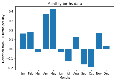
A bar chart may be considered; however, some modifications from the original bar chart are necessary. The values of total births in different months are likely close to each other. A simple bar chart that is showing the absolute values may not present the difference of values very well. Different months have different number of days. It is likely that February has the smallest number, but such a fact does not mean “February is the month that people avoid giving births.”
One suggestion is that we use the number of births per day in a month to represent data.

The following chart is produced with the reflection of modifications.
Show code cell source
# Data initialization
number_births = [253, 229, 247, 251, 261, 239, 244, 252, 235, 242, 245, 249]
days_per_month = [31, 28, 31, 30, 31, 30, 31, 31, 30, 31, 30, 31]
month_labels = ["Jan", "Feb", "Mar", "Apr", "May", "Jun", "Jul", "Aug", "Sep", "Oct", "Nov", "Dec"]

# Transforming the original data of total births to the births by day
births_by_day = []

# Calculating and adding numbers to the list of births by day
for i in range(len(number_births)):
    births_by_day.append(number_births[i] / days_per_month[i])

# Assume that we want to see the difference between a benchmark value, e.g. 8.0, and the actual monthly births
benchmark_number = 8.0
monthly_deviation = []

# Calculating and adding numbers to the list of monthly deviations
for i in range(len(number_births)):
    monthly_deviation.append(births_by_day[i] - 8.0)

# Beginning ploting
import matplotlib.pyplot as plt
import numpy as np

# X: monthly deviation from 8.0 births per day; Y: months
x_months = np.array(month_labels)
y_deviations = np.array(monthly_deviation)

# Displaying the bar chart with labels
plt.bar(x_months, y_deviations)
plt.title("Monthly births data")
plt.xlabel("Months")
plt.ylabel("Deviation from 8.0 births per day")
plt.show()