2.5. Arts in STEM (STEAM)#
Note
The inclusion of arts in STEM is a good way to engage students with diverse interests and abilities. In this chapter, we offer a few examples of a fun way to think about mathematical and programming concepts.
2.5.1. Pixel Images#
Note
In this section, we will show how increasing the number of pixels used to represent an image will sharpen the resolution.
Show code cell source
# PACKAGE: DO NOT EDIT THIS CELL
import numpy as np
import matplotlib
import pandas as pd
matplotlib.use('Agg')
import matplotlib.pyplot as plt
matplotlib.style.use('fivethirtyeight')
from sklearn.datasets import fetch_lfw_people, fetch_olivetti_faces
import time
import timeit
%matplotlib inline
from ipywidgets import interact
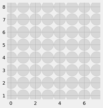
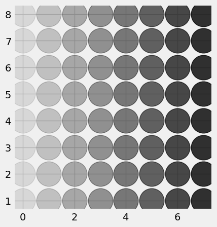
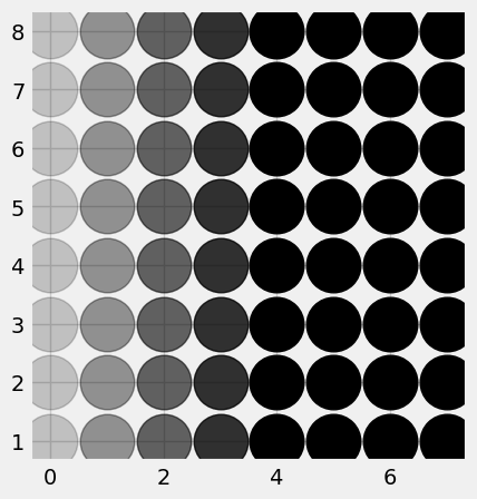
1. Alpha Values The opacity of an image can be adjusted using an alpha value between 0 and 1. For example, a black circle with alpha equal to .1 appears as a light gray and is black when alpha is equal to 1. Note that a rectangular array of alpha values can then be mapped to a rectangular array of circles which have the corresponding shading.
xls=pd.ExcelFile('data.xlsx')
num=3 #number of images
N=8 #NxN pixels
character_collection = {}
for i in np.arange(0,num):
character_collection[i]=pd.read_excel(xls,str(i))
character_collection[0]
| 0 | 1 | 2 | 3 | 4 | 5 | 6 | 7 | |
|---|---|---|---|---|---|---|---|---|
| 0 | 0.1 | 0.1 | 0.1 | 0.1 | 0.1 | 0.1 | 0.1 | 0.1 |
| 1 | 0.1 | 0.1 | 0.1 | 0.1 | 0.1 | 0.1 | 0.1 | 0.1 |
| 2 | 0.1 | 0.1 | 0.1 | 0.1 | 0.1 | 0.1 | 0.1 | 0.1 |
| 3 | 0.1 | 0.1 | 0.1 | 0.1 | 0.1 | 0.1 | 0.1 | 0.1 |
| 4 | 0.1 | 0.1 | 0.1 | 0.1 | 0.1 | 0.1 | 0.1 | 0.1 |
| 5 | 0.1 | 0.1 | 0.1 | 0.1 | 0.1 | 0.1 | 0.1 | 0.1 |
| 6 | 0.1 | 0.1 | 0.1 | 0.1 | 0.1 | 0.1 | 0.1 | 0.1 |
| 7 | 0.1 | 0.1 | 0.1 | 0.1 | 0.1 | 0.1 | 0.1 | 0.1 |
ig=plt.figure(figsize=(4.5,5))
for i in np.arange(0,N):
for j in np.arange(0,N):
plt.plot(j,8-i, marker="o", markersize=35, markeredgecolor='k', markerfacecolor="k",alpha=character_collection[0].loc[i,j])
character_collection[1]
| 0 | 1 | 2 | 3 | 4 | 5 | 6 | 7 | |
|---|---|---|---|---|---|---|---|---|
| 0 | 0.1 | 0.2 | 0.3 | 0.4 | 0.5 | 0.6 | 0.7 | 0.8 |
| 1 | 0.1 | 0.2 | 0.3 | 0.4 | 0.5 | 0.6 | 0.7 | 0.8 |
| 2 | 0.1 | 0.2 | 0.3 | 0.4 | 0.5 | 0.6 | 0.7 | 0.8 |
| 3 | 0.1 | 0.2 | 0.3 | 0.4 | 0.5 | 0.6 | 0.7 | 0.8 |
| 4 | 0.1 | 0.2 | 0.3 | 0.4 | 0.5 | 0.6 | 0.7 | 0.8 |
| 5 | 0.1 | 0.2 | 0.3 | 0.4 | 0.5 | 0.6 | 0.7 | 0.8 |
| 6 | 0.1 | 0.2 | 0.3 | 0.4 | 0.5 | 0.6 | 0.7 | 0.8 |
| 7 | 0.1 | 0.2 | 0.3 | 0.4 | 0.5 | 0.6 | 0.7 | 0.8 |
fig=plt.figure(figsize=(4.5,5))
for i in np.arange(0,N):
for j in np.arange(0,N):
plt.plot(j,8-i, marker="o", markersize=35, markeredgecolor='k', markerfacecolor="k",alpha=character_collection[1].loc[i,j])
character_collection[2]
| 0 | 1 | 2 | 3 | 4 | 5 | 6 | 7 | |
|---|---|---|---|---|---|---|---|---|
| 0 | 0.2 | 0.4 | 0.6 | 0.8 | 1 | 1 | 1 | 1 |
| 1 | 0.2 | 0.4 | 0.6 | 0.8 | 1 | 1 | 1 | 1 |
| 2 | 0.2 | 0.4 | 0.6 | 0.8 | 1 | 1 | 1 | 1 |
| 3 | 0.2 | 0.4 | 0.6 | 0.8 | 1 | 1 | 1 | 1 |
| 4 | 0.2 | 0.4 | 0.6 | 0.8 | 1 | 1 | 1 | 1 |
| 5 | 0.2 | 0.4 | 0.6 | 0.8 | 1 | 1 | 1 | 1 |
| 6 | 0.2 | 0.4 | 0.6 | 0.8 | 1 | 1 | 1 | 1 |
| 7 | 0.2 | 0.4 | 0.6 | 0.8 | 1 | 1 | 1 | 1 |
fig=plt.figure(figsize=(4.5,5))
for i in np.arange(0,N):
for j in np.arange(0,N):
plt.plot(j,8-i,marker="o", markersize=35, markeredgecolor='k', markerfacecolor="k",alpha=character_collection[2].loc[i,j])
2. Pixel Images
We can use Python to create NxN pixel images of a given photo.
For a given black and white picture, a computer code will create an \(N\times N\) array of numbers with gray-scale values.
Or, given an \(N\times N\) array of gray scale values, another computer code can reconstruct a pixel image.
First we install a library for working with pixel images.
!pip install opencv-python
Collecting opencv-python
Downloading opencv_python-4.8.0.74-cp37-abi3-win_amd64.whl (38.1 MB)
0.0/38.1 MB ? eta -:--:--
0.1/38.1 MB 3.5 MB/s eta 0:00:11
0.5/38.1 MB 6.7 MB/s eta 0:00:06
- 1.0/38.1 MB 7.8 MB/s eta 0:00:05
- 1.4/38.1 MB 7.6 MB/s eta 0:00:05
-- 1.9/38.1 MB 8.7 MB/s eta 0:00:05
-- 2.4/38.1 MB 8.6 MB/s eta 0:00:05
--- 2.9/38.1 MB 9.2 MB/s eta 0:00:04
--- 3.3/38.1 MB 9.2 MB/s eta 0:00:04
---- 3.9/38.1 MB 9.5 MB/s eta 0:00:04
---- 4.3/38.1 MB 9.5 MB/s eta 0:00:04
----- 4.9/38.1 MB 9.7 MB/s eta 0:00:04
----- 5.4/38.1 MB 9.8 MB/s eta 0:00:04
------ 5.9/38.1 MB 9.9 MB/s eta 0:00:04
------ 6.4/38.1 MB 10.0 MB/s eta 0:00:04
------- 7.0/38.1 MB 9.9 MB/s eta 0:00:04
------- 7.5/38.1 MB 10.2 MB/s eta 0:00:03
-------- 8.0/38.1 MB 10.1 MB/s eta 0:00:03
-------- 8.5/38.1 MB 10.3 MB/s eta 0:00:03
--------- 9.1/38.1 MB 10.2 MB/s eta 0:00:03
---------- 9.5/38.1 MB 10.2 MB/s eta 0:00:03
---------- 10.1/38.1 MB 10.2 MB/s eta 0:00:03
---------- 10.5/38.1 MB 10.6 MB/s eta 0:00:03
----------- 11.1/38.1 MB 10.7 MB/s eta 0:00:03
----------- 11.7/38.1 MB 10.9 MB/s eta 0:00:03
------------ 12.2/38.1 MB 10.9 MB/s eta 0:00:03
------------- 12.7/38.1 MB 10.9 MB/s eta 0:00:03
------------- 13.2/38.1 MB 10.9 MB/s eta 0:00:03
-------------- 13.7/38.1 MB 10.9 MB/s eta 0:00:03
-------------- 14.3/38.1 MB 11.1 MB/s eta 0:00:03
--------------- 14.8/38.1 MB 11.1 MB/s eta 0:00:03
--------------- 15.4/38.1 MB 11.1 MB/s eta 0:00:03
---------------- 15.9/38.1 MB 10.9 MB/s eta 0:00:03
---------------- 16.4/38.1 MB 11.1 MB/s eta 0:00:02
----------------- 16.9/38.1 MB 11.1 MB/s eta 0:00:02
----------------- 17.4/38.1 MB 10.9 MB/s eta 0:00:02
------------------ 17.9/38.1 MB 10.9 MB/s eta 0:00:02
------------------ 18.5/38.1 MB 10.9 MB/s eta 0:00:02
------------------- 19.0/38.1 MB 11.1 MB/s eta 0:00:02
-------------------- 19.5/38.1 MB 11.1 MB/s eta 0:00:02
-------------------- 20.1/38.1 MB 10.9 MB/s eta 0:00:02
--------------------- 20.5/38.1 MB 11.1 MB/s eta 0:00:02
--------------------- 21.0/38.1 MB 10.9 MB/s eta 0:00:02
--------------------- 21.5/38.1 MB 10.7 MB/s eta 0:00:02
---------------------- 22.0/38.1 MB 10.9 MB/s eta 0:00:02
----------------------- 22.4/38.1 MB 10.7 MB/s eta 0:00:02
----------------------- 23.0/38.1 MB 10.9 MB/s eta 0:00:02
------------------------ 23.5/38.1 MB 10.7 MB/s eta 0:00:02
------------------------ 24.0/38.1 MB 11.1 MB/s eta 0:00:02
------------------------- 24.5/38.1 MB 10.9 MB/s eta 0:00:02
------------------------- 25.0/38.1 MB 10.7 MB/s eta 0:00:02
-------------------------- 25.4/38.1 MB 10.9 MB/s eta 0:00:02
-------------------------- 25.9/38.1 MB 10.7 MB/s eta 0:00:02
--------------------------- 26.5/38.1 MB 10.7 MB/s eta 0:00:02
--------------------------- 27.1/38.1 MB 10.7 MB/s eta 0:00:02
---------------------------- 27.5/38.1 MB 10.7 MB/s eta 0:00:01
---------------------------- 28.1/38.1 MB 10.7 MB/s eta 0:00:01
----------------------------- 28.6/38.1 MB 10.7 MB/s eta 0:00:01
----------------------------- 29.1/38.1 MB 10.6 MB/s eta 0:00:01
------------------------------ 29.6/38.1 MB 10.7 MB/s eta 0:00:01
------------------------------ 30.1/38.1 MB 10.6 MB/s eta 0:00:01
------------------------------- 30.7/38.1 MB 10.6 MB/s eta 0:00:01
------------------------------- 31.2/38.1 MB 10.9 MB/s eta 0:00:01
-------------------------------- 31.7/38.1 MB 10.7 MB/s eta 0:00:01
-------------------------------- 32.2/38.1 MB 10.7 MB/s eta 0:00:01
--------------------------------- 32.7/38.1 MB 10.7 MB/s eta 0:00:01
---------------------------------- 33.2/38.1 MB 10.9 MB/s eta 0:00:01
---------------------------------- 33.7/38.1 MB 10.7 MB/s eta 0:00:01
---------------------------------- 34.1/38.1 MB 10.6 MB/s eta 0:00:01
----------------------------------- 34.7/38.1 MB 10.7 MB/s eta 0:00:01
------------------------------------ 35.2/38.1 MB 10.7 MB/s eta 0:00:01
------------------------------------ 35.7/38.1 MB 10.9 MB/s eta 0:00:01
------------------------------------- 36.2/38.1 MB 10.9 MB/s eta 0:00:01
------------------------------------- 36.8/38.1 MB 10.9 MB/s eta 0:00:01
-------------------------------------- 37.3/38.1 MB 10.7 MB/s eta 0:00:01
-------------------------------------- 37.8/38.1 MB 10.9 MB/s eta 0:00:01
-------------------------------------- 38.1/38.1 MB 10.7 MB/s eta 0:00:01
-------------------------------------- 38.1/38.1 MB 10.7 MB/s eta 0:00:01
---------------------------------------- 38.1/38.1 MB 9.8 MB/s eta 0:00:00
Requirement already satisfied: numpy>=1.21.2 in c:\users\pisihara\appdata\local\anaconda3\lib\site-packages (from opencv-python) (1.24.3)
Installing collected packages: opencv-python
Successfully installed opencv-python-4.8.0.74
Show code cell source
# import libraries
import cv2, os
import numpy as np
import numpy
import pandas as pd
import matplotlib.pyplot as plt
The following function takes a picture file stored in a folder (in our case we will call the folder “images”) and creates an N x N pixel image.
Show code cell source
def makepixelimage(folder, N):
directory = folder
# A data structure called a dictionary is used to store the image data and the dataframes we'll make from them.
imgs = {}
dfs = {}
# Specify the pixel image size
dsize = (N, N)
# This will iterate over every image in the directory given, read it into data, and create a
# dataframe for it. Both the image data and its corresponding dataframe are stored.
# Note that when being read into data, we interpret the image as grayscale.
pos = 0
for filename in os.listdir(directory):
f = os.path.join(directory, filename)
# checking if it is a file
if os.path.isfile(f):
imgs[pos] = cv2.imread(f, 0) # image data
imgs[pos] = cv2.resize(imgs[pos], dsize)
dfs[pos] = pd.DataFrame(imgs[pos]) # dataframe
pos += 1
return plt.imshow(imgs[0], cmap="gray")
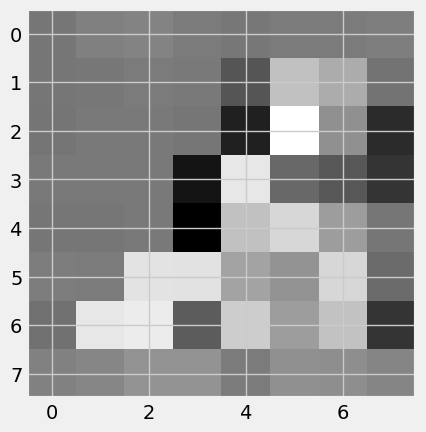
First let’s create an 8x8 pixel image. Can you guess the original picture?
makepixelimage("images", 8)
<matplotlib.image.AxesImage at 0x1e18f71b3d0>
Assignment#
Assignment
1a) By increasing the number of pixels, we can get a better reproduction of the original. Create a 16x16 pixel image. b) Create a 32x32 pixel image.
Upload a different image into a folder called “my_images”. Then use the makepixelimage( , ) function to create an 8x8, 16x16 and 32x32 pixel image and see if the others in the class can guess your original image
2.5.2. Word Clouds#
Note
In this lab, we will create word clouds – artistic representations of words from a speech, book, song or poem. The frequency or number of times a word occurs is represented by the size of that word in the word cloud.
Watch the famous “I have a Dream” speech by Dr. Martin Luther King
“Martin Luther King’s final speech: ‘I’ve been to the mountaintop’” YouTube, uploaded by Guardian News, 4 April 2018, https://youtu.be/e49VEpWg61M?si=2IYOozVbQUfv9SUH. Permissions: YouTube Terms of Service
from IPython.display import YouTubeVideo
YouTubeVideo('o8dzxh7Ybqw', width=800, height=300)
1. Import the Python data analytics (pandas or pd) and numerical Python (numpy) libraries.
Show code cell source
import pandas as pd
import numpy as np
Q1 What is the abbreviation for numpy?
2. Use pandas (pd) to read in the Excel file with the words of the chorus “I have the joy, joy, joy, joy, down in my heart.”
Show code cell source
joy=pd.read_excel("joy.xlsx") #read in the Excel file with the words
joy.head(5) #Display the first 5 rows.
| WORDS | |
|---|---|
| 0 | I |
| 1 | have |
| 2 | the |
| 3 | joy |
| 4 | joy |
Q2 What word is in row 4?
3. Get the frequencies of each word
Show code cell source
joy["WORDS"].value_counts()
joy 8
down 5
in 5
heart 5
my 3
where 3
I 2
have 2
the 2
my 2
to 1
stay 1
Name: WORDS, dtype: int64
Q3 Which word has the highest frequency?
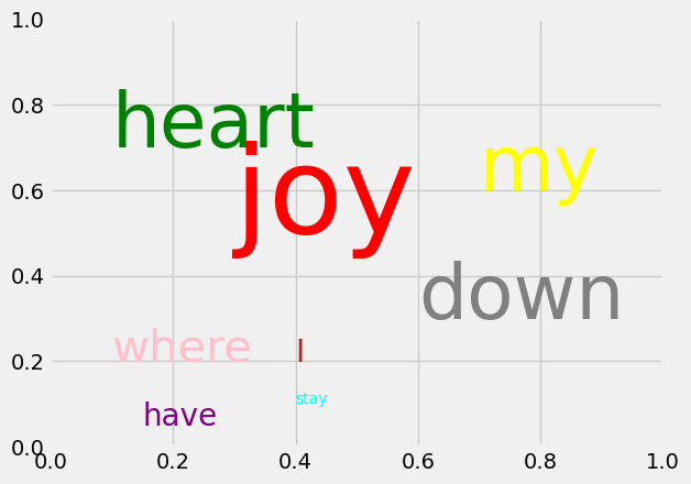
4. We can make a simple word cloud by putting each important word in a specified place, with a given color, and given size. Add the text joy to the word cloud at position .3,.5 in color ‘red’ and fontsize=80.
Show code cell source
from matplotlib import pyplot as plt # library used for making graphs
fig=plt.figure()
plt.gca().text(.3,.5, 'joy',color='red',fontsize=80)
plt.gca().text(.1,.7, 'heart',color='green',fontsize=50)
plt.gca().text(.6,.3, 'down',color='gray',fontsize=50)
plt.gca().text(.7,.6, 'my',color='yellow',fontsize=50)
plt.gca().text(.1,.2, 'where',color='pink',fontsize=30)
plt.gca().text(.4,.2, 'I',color='brown',fontsize=20)
plt.gca().text(.15,.05, 'have',color='purple',fontsize=20)
plt.gca().text(.4,.1, 'stay',color='cyan',fontsize=10)
plt.show()
Q4 What command is used to include the word joy?
5. Data scientists have created functions to make word clouds so we don’t have to enter each word or letter one by one. These are found in the wordcloud library.
!pip install wordcloud
Collecting wordcloud
Downloading wordcloud-1.9.2-cp311-cp311-win_amd64.whl (151 kB)
0.0/151.4 kB ? eta -:--:--
-------------------------------------- 151.4/151.4 kB 4.6 MB/s eta 0:00:00
Requirement already satisfied: numpy>=1.6.1 in c:\users\pisihara\appdata\local\anaconda3\lib\site-packages (from wordcloud) (1.24.3)
Requirement already satisfied: pillow in c:\users\pisihara\appdata\local\anaconda3\lib\site-packages (from wordcloud) (9.4.0)
Requirement already satisfied: matplotlib in c:\users\pisihara\appdata\local\anaconda3\lib\site-packages (from wordcloud) (3.7.1)
Requirement already satisfied: contourpy>=1.0.1 in c:\users\pisihara\appdata\local\anaconda3\lib\site-packages (from matplotlib->wordcloud) (1.0.5)
Requirement already satisfied: cycler>=0.10 in c:\users\pisihara\appdata\local\anaconda3\lib\site-packages (from matplotlib->wordcloud) (0.11.0)
Requirement already satisfied: fonttools>=4.22.0 in c:\users\pisihara\appdata\local\anaconda3\lib\site-packages (from matplotlib->wordcloud) (4.25.0)
Requirement already satisfied: kiwisolver>=1.0.1 in c:\users\pisihara\appdata\local\anaconda3\lib\site-packages (from matplotlib->wordcloud) (1.4.4)
Requirement already satisfied: packaging>=20.0 in c:\users\pisihara\appdata\local\anaconda3\lib\site-packages (from matplotlib->wordcloud) (23.0)
Requirement already satisfied: pyparsing>=2.3.1 in c:\users\pisihara\appdata\local\anaconda3\lib\site-packages (from matplotlib->wordcloud) (3.0.9)
Requirement already satisfied: python-dateutil>=2.7 in c:\users\pisihara\appdata\local\anaconda3\lib\site-packages (from matplotlib->wordcloud) (2.8.2)
Requirement already satisfied: six>=1.5 in c:\users\pisihara\appdata\local\anaconda3\lib\site-packages (from python-dateutil>=2.7->matplotlib->wordcloud) (1.16.0)
Installing collected packages: wordcloud
Successfully installed wordcloud-1.9.2
import wordcloud #used to make a wordcloud
Q5 What is the name of the library which creates word clouds?
6. Check how fast the computer can read the text file with the words to Dr. Martin Luther King’s “I have a dream” speech.
Show code cell source
import time #use to measure time
start = time.time() #record the start time
with open('I have a dream.txt','r') as file: #read in the text file
speech = file.readlines()
finish = time.time() #record the finish time
print(finish - start)
0.009278297424316406
Q6 How fast did the computer read the text file?
7. Define a function to take out punctuation marks and count the interesting words
Show code cell source
#Define a function which counts the interesting words
def calculate_frequencies(textfile):
#list of punctuations
punctuations = '''!()-[]{};:'"\,<>./?@#$%^&*_~'''
#list of uninteresting words
uninteresting_words = ["AND","IT","THE"] #add to this list
# removes punctuation and uninteresting words
import re
fc1=str(textfile)
fc2= fc1.split(' ')
for i in range(len(fc2)):
fc2[i] = fc2[i].upper()
#Remove punctuations
fc3 = []
for s in fc2:
if not any([o in s for o in punctuations]):
fc3.append(s)
#Remove uninteresting words
fc4=[]
for s in fc3:
if not any([o in s for o in uninteresting_words]):
fc4.append(s)
fc5=[]
for s in fc4:
if not any([o.lower() in s for o in uninteresting_words]):
fc5.append(s)
while('' in fc5) :
fc5.remove('')
import collections
fc6 = collections.Counter(fc5)
#wordcloud
cloud = wordcloud.WordCloud( max_words = 30) #can adjust the number of words
cloud.generate_from_frequencies(fc6)
return cloud.to_array()
Q7 What uninteresting words does the above function remove from the word cloud?
8. Make the word cloud by executing the next cell. Then modify the calculate_frequencies() function to eliminate uninteresting words. Also change how many words are displayed.
Show code cell source
myimage = calculate_frequencies(speech)
plt.imshow(myimage, interpolation = 'nearest')
plt.axis('off')
plt.savefig('Ihaveadream.png', bbox_inches='tight')
plt.show()
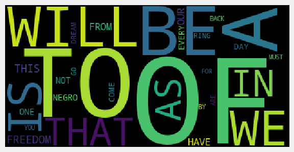
Q8 What is the name of the file with the word cloud image for the “I have a dream” speech?
Assignment#
Assignment
Create word cloud of a famous speech, poem, song etc. Then edit out all the uninteresting words. Then see if the others in the class can figure out your source from 10 words, 20 words, 30 words etc.
2.5.3. Name That Tune!#
Note
In this lab we will explore the basic relationship between sound and a mathematical description of sound using sine waves.
1. Watch the video “Slow-motion Vibrating Guitar String!” YouTube, uploaded by LB’s Epic Tutorials, 23 January 2017, https://youtu.be/tVYQRC1-D54?si=V9ahx88FVM8GXT2i. Permissions: YouTube Terms of Service
and observe that the periodic vibration of a guitar string causes a sound wave.
from IPython.display import YouTubeVideo
YouTubeVideo('tVYQRC1-D54')
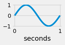
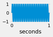
Pure tones can be modelled using sine waves. The amplitude of a sine wave (high high up and down it oscillates) is proportional to the volume of the sound. The frequency of a sine wave is defined as the number of times a wave completes its up and down cycle in one second. The higher the frequency of a sound wave, the higher the pitch. Use the function defined in the next cell to check what happens to a sine wave if we change its frequency.
Show code cell source
import numpy as np
def sinewave(frequency):
#-----------CREATE THE SOUND WAVE-------------------
sampling_rate=44100 #how many times we take a measurement each second
t = np.linspace(0,1,sampling_rate) # take 44100 samples in 1 second;
sound_wave=np.sin(frequency* 2*np.pi* t) # mathematical definition of a sine wave
#----------PLOT THE SOUND WAVE----------------------
import matplotlib.pyplot as plt
fig=plt.figure(figsize=(2,1))
plt.plot(t,sound_wave)
plt.xlabel("seconds")
return
sinewave(1) #frequency=1 and 1 cycle per second
sinewave(2) #frequency=2 and 2 cycles per second
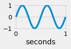
sinewave(3) #frequency=3 and 3 cycles per second
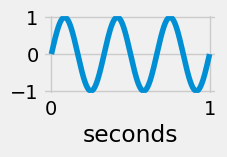
sinewave(20) #frequency=20 and 20 cycles per second
2. If an object vibrates at high enough of a frequency, it creates a sound wave that we can hear. The following function converts a frequency into a sine wave and then into an audible sound
Show code cell source
def play(freq):
import numpy as np
from IPython.display import Audio #library used to create sounds
sampling_rate = 44100 # <- rate of sampling
t = np.linspace(0, 2, sampling_rate) # <- setup time values
sound_wave = np.sin(2 * np.pi * freq * t) # <- sine function formula
return Audio(sound_wave, rate=sampling_rate, autoplay=True) # play the generated sound
play(220) # play a sound at 220 hz
Doubling the frequency creates the same note but an octave higher.
play(440) # play a sound at 440 hz
3. A musical scale can be created by multipling the first note in the scale by different fractions
Show code cell source
import numpy as np
from IPython.display import Audio
rest=0
do=220
re=9/8*220
mi=5/4*220
fa=4/3*220
so=3/2*220
la=5/3*220
ti=15/8*220
do1=2*220
re1=2*9/8*220
mi1=2*5/4*220
fa1=2*4/3*220
so1=2*3/2*220
la1=2*5/3*220
ti1=2*15/8*220
do2=2*2*220
scale=[do,re,mi,fa,so,la,ti,do1]
twooctavescale=[do,re,mi,fa,so,la,ti,do1,re1,mi1,fa1,so1,la1,ti1,do2]
The following function can play a scale or song for us.
Show code cell source
def play(song):
song=np.array(song)
framerate = 44100
t = np.linspace(0, len(song) / 2, round(framerate * len(song) / 2))[:-1]
song_idx = np.floor(t * 2).astype(int)
data = np.sin(2 * np.pi * song[song_idx] * t)
return Audio(data, rate=framerate, autoplay=True)
play(scale)
play(twooctavescale)
4. We can create tunes by arranging notes in a scale.
weshallovercome = [so, so , la, la, so, fa,mi,rest,so, so , la, la, so, fa,mi,rest,so,so,la,ti,do1,do1,re1,re1,ti,la,ti,la,so,so,la,ti,do1,do1,ti,la,so,so,rest,rest,la,la,so,fa,mi,mi,rest,rest,so,so,do,fa,mi,mi,re,re,do,do,do,do,rest,rest]
play(weshallovercome)
Assignment#
Assignment
Create your own tune. When you are finished, see if the others can name that tune!
2.5.4. Random Numbers and Pi#
Note
In this lab we will use random numbers to estimate \(\pi\approx 3.14\).
Let’s look at the library matplotlib. The matplotlib (mpl) library has a sub-library called pyplot (plt). We can access the functions in pyplot by executing the next cell
import matplotlib.pyplot as plt
import numpy as np
np.random.seed(1232023) # The seed determines a specific stream of pseuod random numbers
1. A random number is any number whose decimal is between 0 and 1. Let’s use a random number generator to generate 100 random numbers and then plot them.
N=100
x=np.arange(0,N,1)
y=np.random.rand(N)
plt.scatter(x, y, s=y, marker='o')
<matplotlib.collections.PathCollection at 0x1e1909832d0>
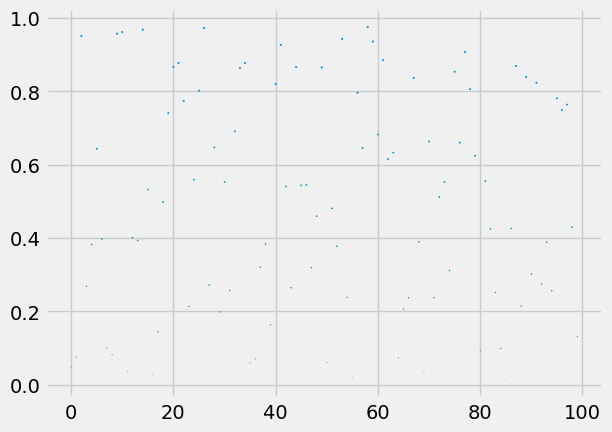
Q1.: How are the 100 random numbers represented in this graph?
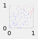
2. Here is a different plot of random numbers.
fig=plt.figure(figsize=(1,1))
N=100
x=np.random.rand(N)
y=np.random.rand(N)
plt.scatter(x, y,s=.1, marker='o')
<matplotlib.collections.PathCollection at 0x1e1909d1290>
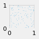
Q2 How were random numbers used to generate the plot above?
3. The distance d from a point (x,y) to the origin (0,0) is given by the formula
Let’s define a function dist(x,y) to compute this distance.
def dist(x,y):
d=np.sqrt(x**2+y**2)
return d
Let’s use our function to check the distance from (3,4) to the origin.
Show code cell source
dist(3,4)
Q3a What is the distance between (8,15) and the origin?
Q3b Can you find another pair of non-zero integers (a,b) whose distance to the origin is another integer c? (The integers a,b,c are called a “Pythagorean triple”)
4. Let’s use random numbers to create a plot of points in blue if the distance is less than or equal to 1 and in red if the distance is more than 1.
Show code cell source
fig=plt.figure(figsize=(1,1))
for n in np.arange(0,1000,1):
x=np.random.rand(1)
y=np.random.rand(1)
if dist(x,y)<=1:
plt.scatter(x, y,s=.1, marker='o', color='blue')
else:
plt.scatter(x, y,s=.1, marker='o', color='red')
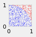
Q4 What is the shape of the points in blue?
5. The area \(A\) of a circle with radius \(r\) is \(A=\pi r^2\).
Q5 What is the area of a quarter circle of radius \(r=1\)?
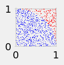
6. Note that \(\pi/4\approx .785\). Thus, we would expect about 78.5% of the points in the plot in Step 4 to be in blue. Let’s check this by counting the number of points of each color plotting a total of \(N=100\) points.
Show code cell source
fig=plt.figure(figsize=(1,1))
N=100
blue=0
red=0
for n in np.arange(0,N,1):
x=np.random.rand(1)
y=np.random.rand(1)
if dist(x,y)<=1:
plt.scatter(x, y,s=.1, marker='o', color='blue')
blue=blue+1
else:
plt.scatter(x, y,s=.1, marker='o', color='red')
red=red+1
print("Percentage of Blue Points=", (blue/N)*100)
print("Estimate of Pi=", 4* (blue/N))
Percentage of Blue Points= 80.0
Estimate of Pi= 3.2
Q6 What would the approximation of pi be if the percentage of blue points had been 81?
7. Let’s see what happens if we use \(N=1000\).
Show code cell source
fig=plt.figure(figsize=(1,1))
N=1000
blue=0
red=0
for n in np.arange(0,N,1):
x=np.random.rand(1)
y=np.random.rand(1)
if dist(x,y)<=1:
plt.scatter(x, y,s=.1, marker='o', color='blue')
blue=blue+1
else:
plt.scatter(x, y,s=.1, marker='o', color='red')
red=red+1
print("Percentage of Blue Points=", (blue/N)*100)
print("Estimate of Pi=", 4* (blue/N))
Percentage of Blue Points= 79.3
Estimate of Pi= 3.172
7. What is happening to the percentage of blue points as we increase \(N\) from 100 to 1000?
Assignment#
Assignment
What do you expect to happen if we increase \(N\) to 5,000?
Check to see if you are correct.
2.5.5. Simulating Formula 1#
Note
In this section, we will use an object oriented approach to create a simple animation of formula 1 cars turning a corner.
1. First we import libraries.
Show code cell source
import matplotlib.pyplot as plt
import matplotlib.image as mpimg
from matplotlib.offsetbox import TextArea, DrawingArea, OffsetImage, AnnotationBbox
import numpy as np
import scipy.misc
from scipy import ndimage
from PIL import Image
import numpy as np
import pandas as pd
import matplotlib.animation as animation
from matplotlib.animation import FuncAnimation
%matplotlib notebook
2. Next we create a car class. A class is a special programming tool similar to a function, but with additional features.
Each car has properties or attributes including:
x position
y position
an image file showing what the car looks like
a size (which can be adjusted)
speed
Each car also has a method which is a type of function.
go
class car:
def __init__(self,x,y,image,size,speed): #properties
self.x=x #object's position is (x,y)
self.y=y
self.image=image #name of the image file
self.size=size
self.speed=speed
def go(self,xamount,yamount): #method to move the object vertically
self.x=self.x+xamount*self.speed
self.y = self.y+yamount*self.speed
return
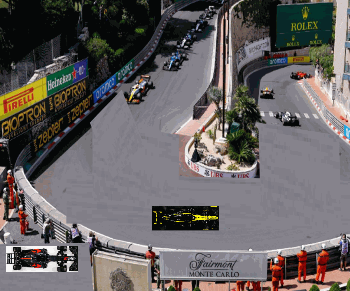
3. We’ll define a function which positions two cars on a track.
Show code cell source
#create a function to position the cars on the track
def simulate(c1,c2,n):
#make a graph
fig = plt.figure(figsize=(12,10))
plt.gca().set_aspect('equal')
ax = plt.axes([0.1, 0.1, 1, 1])
#add a track diagramimagebox = OffsetImage(simulation, zoom=1)
simulation = mpimg.imread('monaco.png')
imagebox = OffsetImage(simulation, zoom=1)
ab = AnnotationBbox(imagebox, (0.5, 0.45),frameon=False)
plt.gca().add_artist(ab)
car1 = mpimg.imread(c1.image)
imagebox= OffsetImage(car1, zoom=c1.size)
firstcar = AnnotationBbox(imagebox, (c1.x, c1.y),frameon=False)
plt.gca().add_artist(firstcar)
car2 = mpimg.imread(c2.image)
imagebox= OffsetImage(car2, zoom=c2.size)
secondorn = AnnotationBbox(imagebox, (c2.x, c2.y),frameon=False)
plt.gca().add_artist(secondorn)
plt.savefig(str(n)+'.png')
plt.show()
return
4. We’ll create two car objects and use our function to position the yellow car on the track (frame 1 of our animation).
c1=car(.43,.15,'car1.png',.14,0)
c2=car(.02,.01,'car2.png',.12,0)
simulate(c1,c2,0)
5. We’ll use the go method to move the yellow car forward (frame 2 of the animation).
c1.speed=.8
c1.go(.2,0)
simulate(c1,c2,1)
6. We’ll show the yellow car after it turns the corner (frame 3 of the animation).
c1.speed=.9
c1.size=c1.size*.9
c1.go(.2,.15)
c1.image="car1left.png"
simulate(c1,c2,2)
7. Now let’s put the three frames together into an animation “F1.gif”
Show code cell source
frames=3
from PIL import Image
images = []
for n in range(frames):
exec('a'+str(n)+'=Image.open("'+str(n)+'.png")')
images.append(eval('a'+str(n)))
images[0].save('F1.gif',
save_all=True,
append_images=images[1:],
duration=300,
loop=0)
Assignment#
Assignment
Put the red car onto the track right and show it following right behind the yellow car around the turn. Then create an animation called “F1a.gif”.