7.7. Related Rates with Trig Functions and Football

In this lab, we will solve a related rates problem which involves the use of trig functions. In particular, we will determine how fast a camera is rotating as it tracks a football player speeding along the sideline to the endzone.

The following code creates the animation, Football_Animation.gif. If you execute the code, you can open and view the .gif file.

Show code cell source Hide code cell source

import numpy as np
import pandas as pd
import matplotlib.pyplot as plt
from matplotlib.path import Path
import matplotlib.animation as animation
from matplotlib.animation import FuncAnimation
%matplotlib notebook
%matplotlib inline
from matplotlib.markers import MarkerStyle
import matplotlib.pyplot as plt
from matplotlib.lines import Line2D
from matplotlib.transforms import Affine2D
import matplotlib.patches as patches
from matplotlib.patches import Rectangle

frames=9
for n in range(frames):

#green background
    verts = [(-20, -20),  # left, bottom
         (-20, 100),  # left, top
         (100, 100),  # right, top
         (100, -20),  # right, bottom
         (0., 0.),  # ignored
        ]
    codes = [Path.MOVETO,Path.LINETO,Path.LINETO,Path.LINETO,Path.CLOSEPOLY,]

    path = Path(verts, codes)
    patch = patches.PathPatch(path, facecolor='green', lw=.1, edgecolor='w')
    fig, ax = plt.subplots()
    ax.add_patch(patch)
    ax.set_xlim(-2, 10)
    ax.set_ylim(-2, 10)
    
#endzone
    plt.gca().add_patch(Rectangle((7.88,-20),50,20.04, edgecolor='w', facecolor=(.0,.1,.4), lw=4))

#side line
    plt.gca().add_patch(Rectangle((6.8,-20),70,200, edgecolor='w', facecolor='none', lw=70))

#Yard Marks
    yards= [0,1,2,3,4,5,6,7,8,9,10]
    for i in range(len(yards)):
        plt.gca().add_patch(Rectangle((8.1,i),.5,.1, edgecolor='w', facecolor='w', lw=1))
#5 & 10
    plt.gca().add_patch(Rectangle((8.1,5),50,.1, edgecolor='w', facecolor='w', lw=1))
    plt.gca().add_patch(Rectangle((8.1,10),50,.1, edgecolor='w', facecolor='w', lw=1))

#Adjacent line to camera
    plt.gca().add_patch(Rectangle((0.3,-0.1),7.68,.1, edgecolor='none', facecolor='yellow', lw=1))

#Tracking line
    x = np.linspace(0, 8, 100)
    f = lambda x : ((8-n)/8)*x
    y=f(x)
    plt.plot(x,((8-n)/8)*x,'--y')

#Bob Hayes
    import matplotlib as mpl
    from svgpath2mpl import parse_path
    from svgpathtools import svg2paths
    player_path, attributes = svg2paths('bullet_bob.svg')
    player_marker = parse_path(attributes[0]['d'])
    player_marker.vertices -= player_marker.vertices.mean(axis=0)
    x=7.8
    y=8.8-(n)
    plt.plot(x,y, marker=player_marker, markersize=35,color= 'b')
    
#Camera
    camera_path, attributes = svg2paths('camera.svg')
    camera_marker = parse_path(attributes[0]['d'])
    camera_marker.vertices -= camera_marker.vertices.mean(axis=0)
    camera_marker = camera_marker.transformed(mpl.transforms.Affine2D().rotate_deg(45-(5*n)))
    camera_marker = camera_marker.transformed(mpl.transforms.Affine2D().scale(.1,.1))
    x = -0.01
    y = 0.15
    plt.plot(x,y,marker=camera_marker,markersize=30,color = 'k')

#Annotations
    ax.annotate('Camera',
                xy=(0, 1), xycoords='data',
                xytext=(0, -35), textcoords='offset points', color='white')
#Legend
    plt.xlabel('Distance from camera (yds)')
    plt.ylabel('Distance from endzone (yds)')
    plt.title('"Bullet" Bob Hayes Returning a Kick')

#Save each frame as a .png
    plt.savefig(str(n)+'.png')
    plt.close()

#Save as a GIF
from PIL import Image
images = []
for n in range(frames):
    exec('a'+str(n)+'=Image.open("'+str(n)+'.png")')
    images.append(eval('a'+str(n)))
images[0].save('Football_Animation.gif',
               save_all=True,
               append_images=images[1:],
               duration=400,
               loop=0)

Now the idea of the scenario is how we can use calculus to solve the problem of how fast the camera must rotate to stay pointed at the player. To begin, we need to review some basic info about trig functions.

7.7.1. Definition of Trig Functions

The acronym SOH-CAH-TOA is helpful to remember the definitions of the three basic trig functions sine, cosine, and tangent as ratios of sides of a right triangle:

\[\sin(\theta)=\frac{opposite}{hypotenuse}\]

\[\cos(\theta)=\frac{adjacent}{hypotenuse} \]

\[\tan(\theta)= \frac{opposite}{adjacent} \]

7.7.2. Derivatives of basic trig functions

The basic derivative formulas are

\[ \frac{d}{d\theta} \sin(\theta)=\cos(\theta) \]

\[\frac{d}{d\theta} \cos(\theta)=-\sin(\theta) \]

\[ \frac{d}{d\theta} \tan(\theta)=\sec^2(\theta)=\frac{1}{\cos^2(\theta)} \]

In our application problem, we will assume that the angle \(\theta\) is changing with time \(t\). In this case, the derivatives with respect to time \(t\) are given by

\[\frac{d}{dt}\sin(\theta(t))=\cos(\theta)\frac{d\theta}{dt}\]

\[\frac{d}{dt}\cos(\theta(t))=-\sin(\theta)\frac{d\theta}{dt}\]

\[\frac{d}{dt}\tan(\theta(t))=\sec^2(\theta)\frac{d\theta}{dt}=\frac{d\theta/dt}{\cos^2(\theta)} \]

Example

Find \(\frac{d}{dt}\) of \(\tan\)(\(t^2\)). (Hint: In this case, \(\theta(t)=t^2\))

Answer: \(\sec^2(t^2)2t\) or \(\frac{2t}{\cos^2(t^2)}\)

Explanation:

It’s been given that the derivative \(d/dt\) of \(\tan\)(\(\theta(t)\)) is \(\sec^2(\theta)\frac{d\theta}{dt}\) . Therefore, since \(d\theta/dt\) is \(2t\), multiplying by \(\sec^2(\theta)\) gives \(\sec^2(t^2)2t\) or equivalently, \(\frac{2t}{\cos^2(t^2)}\).

7.7.3. Radian Measure

The above formulas for the derivatives of \(\sin(\theta)\), \(\cos(\theta))\) and \(\tan(\theta)\) all assume that the angle \(\theta\) is measured in radians.

Conversion between radians and degrees is possible if we remember that \(\pi\) radians = 180 degrees or \(2\pi\) radians = 360 degrees.

Example

Convert \(\frac{5}{6}\) radians to degrees

Answer: \(\frac{5}{6}\) \(radians\) x \(\frac{180 \, degrees}{\pi \, radians}\) = \(\frac{150}{\pi}\) degrees

Explanation:

It’s been given that \(\pi\) radians = 180 degrees so \(\frac{180 \, degrees}{\pi \, radians} = 1\). We can complete the conversion using cross cancellation method.

7.7.4. Python trig functions

from math import pi, sin, cos, tan, asin, acos, atan, radians, degrees

You can use these imported python functions to do calculations within the notebook. For correct syntax, code as follows:

sin(pi/4)

0.7071067811865475

To convert from radians to degrees, simply type degrees(radian value). This will give you the corresponding degree value:

degrees(pi)

180.0

Furthermore, by default Python assumes the input angle measure is in radians. You can convert the final answer to degrees as such:

degrees(atan(1)) 

45.0

Note that the above example asks for the degree conversion of the radian value of the arctangent of a right triangle with congruent sides (8/8, 6/6, and so on).

Example

Bob Hayes won the 100 meter dash at the Tokyo ‘64 Olympics equaling the world record of 10.0 seconds. Hayes went on to be a star wide receiver with the Dallas Cowboys.

Suppose a TV camera is positioned on the goal line and 8 yards from the sideline. The camera stays fixed on Hayes, who is currently on the 8 yard line and sprinting towards the end zone at 10 yards per second.

Answer the questions below to determine how fast the camera is turning (in degrees per second).

1. From the Figure below , give an equation for \(y\) in terms of \(\theta\).

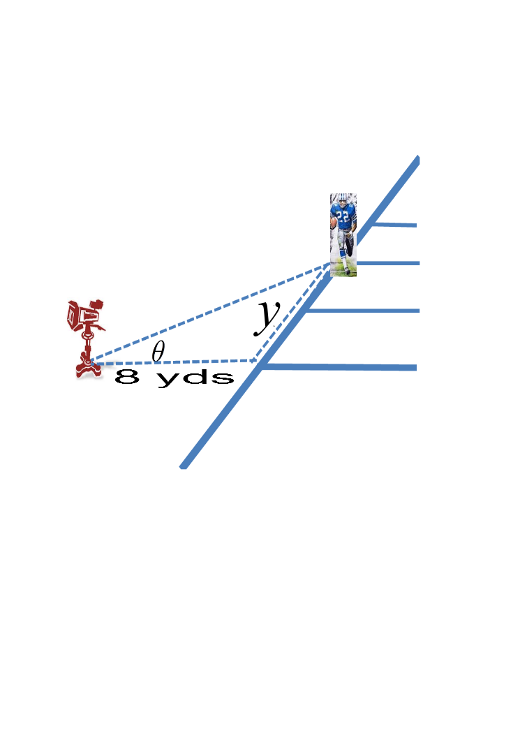
Answer: \(y(t) = 8 \tan(\theta(t)\))

Explanation:

We know that \(\tan(\theta)= \frac{opposite}{adjacent} \).

In our case, the opposite side is \(y\) and adjacent side is 8, so \(\tan\)(\(\theta\)) = \(\frac{y}{8}\).

To convert to \(y(t)\), we multiply on both sides and get \(y(t)\) = \(8\) \(\tan\)(\(\theta\))

2a) What is the physical meaning of \(\frac{dy}{dt}\) ?

Answer: The physical meaning of \(\frac{dy}{dt}\) is the speed of Bob Hayes as he is running towards the end line from the side line measured in yds/sec. A negative value indicates he is getting closer to the goal line.

2b) What is the physical meaning of \(\frac{d\theta}{dt}\) ?

Answer: The physical meaning of \(\frac{d\theta}{/dt}\) is how fast the camera angle is turning as it keeps pointing at Hayes as he runs towards the goal line. A negative value indicates clockwise rotation.

3. If \(\theta\) is measured in radians, then \(\frac{d}{dt} \tan(\theta(t)) = \frac{1}{\cos^2\theta} \frac{d\theta}{dt}\). Use your answer to problem 1 to find a general relationship between \(\frac{dy}{dt}\) and \(\frac{d\theta}{dt}\).

Answer: If \(y = 8\tan(\theta)\), then \(dy/dt = 8\frac{ d\theta/dt}{\cos^2(\theta)}\)

Explanation:

We learn that the derivative of \(tan(\theta) = \frac{1}{\cos^2\theta}\) .

Using chain rule, we deduce that the derivative of \(tan(\theta(t))= \frac{1}{\cos^2\theta}\frac{d\theta}{dt}\) .

Thus, \(\frac{dy}{dt}\), using the equation in question one in which \(y(t) = 8\tan(\theta(t))\), equals \(8 \frac{d(\theta)/dt} {\cos^2(\theta)}\)

4. Find \(\frac{d\theta}{dt}\) (in radians per second) at the instant when \(y=8.\) (Hint: \(\cos(\theta)=\frac{adjacent}{hypotenuse}\)).

Answer: \(-\)\(\frac{5}{8}\)

Explanation:

\[ y(t) = 8 \tan(\theta(t)) \Rightarrow \tan(\theta(t)) = \frac{y(t)}{8}. \]

Since \(y(t) = 8\), then \(\tan(\theta(t)) = 1\), which means \(\theta(t)\) is \(\frac{\pi}{4}\) radians .

The formula

\[ \frac{dy}{dt} = \frac{\frac{d\theta}{dt}}{\cos^2(\theta)} \]

implies that

\[ \frac{d\theta}{dt} = \frac{\cos^2(\theta)\frac{dy}{dt}}{8}. \]

We can substitute \(\theta\) with \(\frac{\pi}{4}\) and \(\frac{dy}{dt}\) with -10.

Then we get:

\[ -\frac{10 \cos^2 (\frac{\pi}{4})}{8} = - \frac{5}{4}\cos^2(\frac{\pi}{4}) = - \frac{5}{4} (\frac{\sqrt 2}{2})^2 = - \frac{5}{4} * \frac{1}{2} = -\frac{5}{8}. \]

5. Use the fact that 1 radian = \((\frac{180}{\pi})^o\) to express your answer to problem 4 in degrees per second.

Answer: \(-\)\(\frac{225}{2\pi}\) degrees per second or around 35.8 degrees per second.

Explanation:

Multiply \(-\frac{5}{8}\frac{ radians}{ second}\) by \(\frac{180 \, degrees}{\pi \, radians} = \frac{225 \, degrees}{2\pi \, seconds}\) = \(-35.8\) degrees per second.

6. Let \(R\) be your answer to problem 5. If the camera revolves at the constant rate of \(R\) degrees per second, how many seconds would it take to make one \(360^o\) revolution?

Answer: It will take the camera approximately 10 seconds to make a full revolution.

Explanation:

Using the cross-canceling unit method, \((360 degrees) \, {\frac{1\ second}{R\ degrees}},\) we cancel the degrees and we are given seconds: \(360/35.8 = 10.04\) seconds.

Questions

1. Find \(\theta\) in degrees if the camera was 3.5 yds from the sidelines.

2. If the camera is rotated .5 radians away from the endzone towards Bob Hayes, what yard line must he be on? (Given he is running at velocity of 10yds/sec again).

3. Find \(\theta\) in radians when t = 0.4 seconds.

4. Find \(\frac{d\theta}{dt}\) in degrees/sec if Bob Hayes had pulled his hamstring and could only run 6 yds/sec at the instant when y=5.

5. Find \(\frac{d\theta}{dt}\) in radians/sec of the angle relative from Bob to the camera when y=4 and he was going 9 yds/sec.

7.7.5. Exercises

Hint: draw pictures to assist you in visualizing the problem and marking necessary measurements.

Exercises

1. A baseball diamond is a square with side length of 90ft. A batter hits the ball and runs toward first base with a speed of 20ft/s. At what rate is his distance from second base decreasing when he is halfway to the first base? At what rate is his angle to second base changing?

2. At 1:00 PM, Jet-ski A is 7 miles east of Jet-ski B. Jet-ski A is moving north at 20 miles/hr while Jet-ski B is moving south 30 miles/h. How fast is the distance between the Jet-skis changing at 3:00 PM?