7.9. Normal Distribution and Process Control

In this lab, we will apply the Normal distribution to statistical process control. The main goal of the latter is to ensure the output of a manufacturing process remains within limits determined by usual random variation. If a very low probability event occurs, this may be used as a signal that there is a problem with the manufacturing process, in which case the process might be stopped and equipment checked for possible defects.

Derivatives of Exponential Functions

The normal distribution is given by

\[f(x)=\frac{1}{\sigma\sqrt{2\pi}}e^{-\frac{(x-\mu)^2}{2\sigma^2}},\]

where \(\mu\) is a constant called the mean and \(\sigma\) is another constant called the standard deviation.

To analyze the normal distribution using calculus, we need the derivative formula

\[\frac{d}{dx} e^{u(x)}= e^{u(x)}u'(x).\]

For example, let \(f(x) = c_1 e^{-\frac{(x-c_2)^2}{2c_3^2}}\). Then,

\[f'(x)= c_1 e^{-\frac{(x-c_2)^2}{2c_3^2}} [\frac{-2(x-c_2)}{2c_3^2}]=c_1 e^{-\frac{(x-c_2)^2}{2c_3^2}} [\frac{-(x-c_2)}{c_3^2}]\]

Note that \(f'(c_2)=0\). Since \(f'(x)>0\) (\(f\) is increasing) for all \(x<c_2\) and \(f'(x)<0\) (\(f\) is decreasing) for all \(x>c_2\), we know \(f(x)\) has an absolute maximum value at \(x=c_2\).

We use the product rule to find \(f''(x)\):

\[ f''(x)= c_1 e^{-\frac{(x-c_2)^2}{2c_3^2}} [\frac{-(x-c_2)}{c_3^2}]^2+c_1 e^{-\frac{(x-c_2)^2}{2c_3^2}}(-\frac{1}{c_3^2})\]

\[= c_1 e^{-\frac{(x-c_2)^2}{2c_3^2}}[\frac{(x-c_2)^2}{c_3^4}-\frac{1}{c_3^2}].\]

To find the \(x\)-coordinates of the two inflection points, set \(f''(x)=0\):

\[\frac{(x-c_2)^2}{c_3^4}-\frac{1}{c_3^2}=0 \Rightarrow\]

\[\frac{(x-c_2)^2}{c_3^4}= \frac{1}{c_3^2}\Rightarrow \]

\[(x-c_2)^2 = c_3^2 \Rightarrow x-c_2= \pm c_3 \Rightarrow\]

\[x=c_2\pm c_3.\]

The inflection points occur symmetrically about the maximum point at \(x=c_2\).

Rule of 68-95-99.7

If data points are normally distributed,

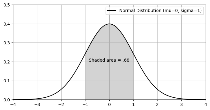
68% of the data will be within 1 standard deviation of the mean,

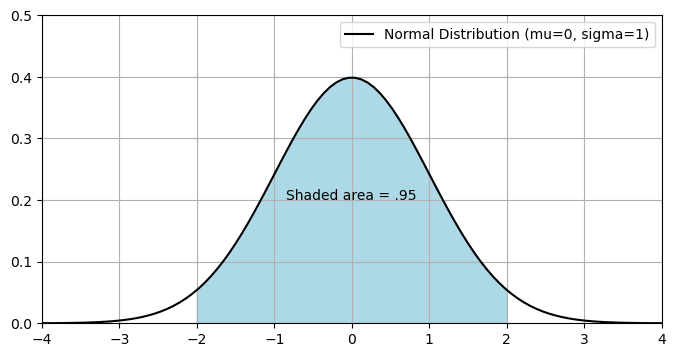
95% of the data will be within 2 standard deviations of the mean, and

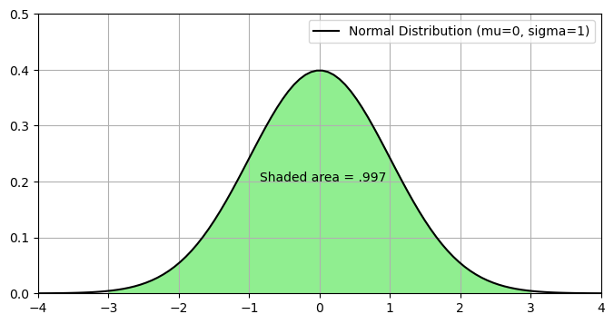
99.7% of the data will be within 3 standard deviations of the mean.

The plot below shows the standard normal distribution with mean \(\mu=0\) and standard deviation \(\sigma=1\). The total area under the curve is equal to 1. The shaded area on the graph below represents the probability that standard normally distributed data will be within 1 standard deviation of the mean.

Show code cell source Hide code cell source

import pandas as pd
import numpy as np
import matplotlib.pyplot as plt
x = np.linspace(-4,4,100)
f= (1/np.sqrt(2*np.pi))*np.exp(-x**2/2)  #standard (unit) normal distribution
plt.figure(figsize=(8, 4))
plt.plot(x,f,color='k',label="Normal Distribution (mu=0, sigma=1)")
plt.xlim((-4.,4))
plt.ylim((0,.5))
x1=np.linspace(-1,1,50)
y1= (1/np.sqrt(2*np.pi))*np.exp(-x1**2/2) 
plt.fill_between(x1,y1,color='lightgray')
plt.text(-.85,.2,'Shaded area = .68')
plt.grid()
plt.legend()
plt.show()

Show code cell source Hide code cell source

x = np.linspace(-4,4,100)
f= (1/np.sqrt(2*np.pi))*np.exp(-x**2/2)  #standard (unit) normal distribution
plt.figure(figsize=(8, 4))
plt.plot(x,f,color='k',label="Normal Distribution (mu=0, sigma=1)")
plt.xlim((-4.,4))
plt.ylim((0,.5))
x2=np.linspace(-2,2,50)
y2= (1/np.sqrt(2*np.pi))*np.exp(-x2**2/2) 
plt.fill_between(x2,y2,color='lightblue')
plt.text(-.85,.2,'Shaded area = .95')
plt.grid()
plt.legend()
plt.show()

Show code cell source Hide code cell source

x = np.linspace(-4,4,100)
f= (1/np.sqrt(2*np.pi))*np.exp(-x**2/2)  #standard (unit) normal distribution
plt.figure(figsize=(8, 4))
plt.plot(x,f,color='k',label="Normal Distribution (mu=0, sigma=1)")
plt.xlim((-4.,4))
plt.ylim((0,.5))
x3=np.linspace(-3,3,50)
y3= (1/np.sqrt(2*np.pi))*np.exp(-x3**2/2) 
plt.fill_between(x3,y3,color='lightgreen')
plt.text(-.85,.2,'Shaded area = .997')
plt.grid()
plt.legend()
plt.show()

7.9.1. Exercises

Exercises

Suppose a manufacturing process of a certain part is “in control” when a sample is normally distributed with average length \(\mu=1\) inch (mean) and standard deviation \(\sigma=.01\) inch.

1. Make a sketch of a normal distribution with this mean and standard deviation, showing the rule of 68-95-99.7.

2. Answer the following:

a) Out of 100 samples, how many would we expect to have an average length between .997 and 1.003 inches?

b) Out of 100 samples, how many would we expect to have an average length of less than .997 inches?

c) Out of 100 samples, how many would we expect to have an average length of less than 1.003 inches?

3. Consider the following sequence of twenty average sample lengths:

1.001, .9995, 1.000, 1.001, 1.002, .998, .999, 1.0025, .9975, .9825, 1.0025, 1.00075, 1.000, .999, .9985, 1.0035, 1.001, 1.000, 1.0015

a) Complete the control chart corresponding to these sample sizes. The outer boundary lines are within 3 standard deviations of the mean. If a data point goes outside these boundaries, this signals the process may be out of control.

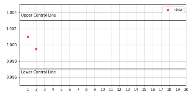
b) Suppose the process is stopped if the average sample length has a probability of less than .0015 of occurring. Will the process be stopped? If so, at what point(s)?

4. A normal distribution with mean \(\mu\) and standard deviation \(\sigma\) is given by

\[ f(x) = \frac{1}{\sigma\sqrt{2\pi}} e^{-\frac{(x-\mu)^2}{2\sigma^2}}\]

where \(\mu\) is the mean and \(\sigma\) the standard deviation \(\sigma>0\)

Use the first and second derivatives to find the exact coordinates of the max/min and inflection points of this exponential function if \(\mu = 1\) and \(\sigma = 0.01\).

Reference: Wayworld.Inc tutorial on Statistical Process Control (SPC) (http://www.wayworld.com/spc/spc.cfm).