4.4. Solutions to Part I Exercises

import pandas as pd
import numpy as np
import matplotlib.pyplot as plt

# Load the data
data = pd.read_csv('census_income.csv')

Exercise 2.1

data.tail()

	age	workclass	fnlwgt	education	education-num	marital-status	occupation	relationship	race	sex	capital-gain	capital-loss	hours-per-week	native-country	income
32556	27	Private	257302	Assoc-acdm	12	Married-civ-spouse	Tech-support	Wife	White	Female	0	0	38	United-States	<=50K
32557	40	Private	154374	HS-grad	9	Married-civ-spouse	Machine-op-inspct	Husband	White	Male	0	0	40	United-States	>50K
32558	58	Private	151910	HS-grad	9	Widowed	Adm-clerical	Unmarried	White	Female	0	0	40	United-States	<=50K
32559	22	Private	201490	HS-grad	9	Never-married	Adm-clerical	Own-child	White	Male	0	0	20	United-States	<=50K
32560	52	Self-emp-inc	287927	HS-grad	9	Married-civ-spouse	Exec-managerial	Wife	White	Female	15024	0	40	United-States	>50K

Exercise 2.2: Answers will vary depending on what students hypothesize each variable to be.

Exercise 2.3:

#remove N/A rows
data = data.dropna()
data.describe()

	age	fnlwgt	education-num	capital-gain	capital-loss	hours-per-week
count	30162.000000	3.016200e+04	30162.000000	30162.000000	30162.000000	30162.000000
mean	38.437902	1.897938e+05	10.121312	1092.007858	88.372489	40.931238
std	13.134665	1.056530e+05	2.549995	7406.346497	404.298370	11.979984
min	17.000000	1.376900e+04	1.000000	0.000000	0.000000	1.000000
25%	28.000000	1.176272e+05	9.000000	0.000000	0.000000	40.000000
50%	37.000000	1.784250e+05	10.000000	0.000000	0.000000	40.000000
75%	47.000000	2.376285e+05	13.000000	0.000000	0.000000	45.000000
max	90.000000	1.484705e+06	16.000000	99999.000000	4356.000000	99.000000

Since we dropped a small proportion of rows, we should not see too many changes in the summary statistics.

Exercise 2.4:

#for the education column
#print out the categories in the column
#then the number of instances for each category
print(data['education'].value_counts())

 HS-grad         9840
 Some-college    6678
 Bachelors       5044
 Masters         1627
 Assoc-voc       1307
 11th            1048
 Assoc-acdm      1008
 10th             820
 7th-8th          557
 Prof-school      542
 9th              455
 12th             377
 Doctorate        375
 5th-6th          288
 1st-4th          151
 Preschool         45
Name: education, dtype: int64

Exercise 2.5:

#function get_value_counts that takes in a variable name (string)
#and returns the value counts for that
def get_value_counts(var_name):
    return data[var_name].value_counts()

#test
print(get_value_counts('occupation'))

 Prof-specialty       4038
 Craft-repair         4030
 Exec-managerial      3992
 Adm-clerical         3721
 Sales                3584
 Other-service        3212
 Machine-op-inspct    1966
 Transport-moving     1572
 Handlers-cleaners    1350
 Farming-fishing       989
 Tech-support          912
 Protective-serv       644
 Priv-house-serv       143
 Armed-Forces            9
Name: occupation, dtype: int64

Exercises 3.1-3.4: Answers will vary depending on the chosen variable, but the code should follow the examples given in the section and the plots should be readable.

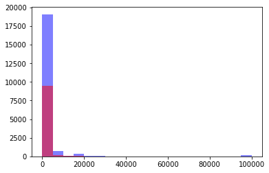
Exercise 3.5:

#split capital-gain by sex
m = data[data['sex'] == " Male"]['capital-gain']
f = data[data['sex'] == " Female"]['capital-gain']

#we are going to plot the histograms of the capital
#with a different color for each sex
plt.hist(m, bins=20, alpha=0.5, color='b')
plt.hist(f, bins=20, alpha=0.5, color='r')
plt.show()

Interpretation of this may vary. An example is that the difference seems to largely be due to one single outlier male with lots of capital gain.

Exercise 3.6: Answers may vary depending on the variables chosen but should follow the example code and the plotting above.

Exercise 3.7: No, the test shows us that there is a difference, but it does not tell us where that difference lies.

Exercise 3.8: Answers may vary depending on the variables chosen but should follow the example code.