7.8. Probability Distributions and Drive Thrus#
7.8.1. Introduction#
Introduction
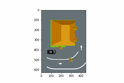
In this section, we show how random numbers are used to simulate a fast-food restaurant with a drive-thru order window as illustrated in the animation below.
For an explanation of how to create this animation, see the “Introduction to Python” section in the Python Programming Guide
For Discussion
Suppose you are the owner of a fast-food restaurant. Currently, there is one drive-thru lane, but you are considering adding a second drive-thru lane. What factors need to be considered in deciding whether to add a second drive-thru lane?
A statistical simulation model uses data of customer arrival and ordering times to re-create a scenario and explore options such as adding a second drive-thru lane. (For example, see the video
“Fast Food Drive Thru 2 lanes versus 1” YouTube, uploaded by Daniel Hickman, 5 March 2013, https://www.youtube.com/watch?v=M9v6bx3l4Dk. Permissions: YouTube Terms of Service
Calculus is used in statistically-based simulations since probabilities are represented as areas under curves called probability distributions.
Here we will focus on the use of uniform (constant) and exponential distributions to model arrival times of customers.
7.8.2. Distributions#
A computer simulation of 1 versus 2 drive-thru lanes uses probabilities computed using definite integrals. The probability that some timed event \(X\) occurs between \(t=a\) and \(t=b\) is given by
\(prob(a\le X \le b) =\int_a^b f(t)\, dt\)
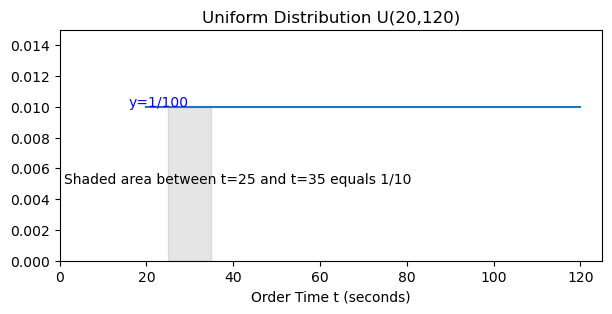
Example 1 Suppose the time to place an order is given by a uniform distribution \(U(20,120)\). In this case, \(f(t)=\frac{1}{100}\) where \(20\le t\le 120\). Find the probability that the length of the next order is between 25 and 35 seconds.
Solution: probability=\(\int_{25}^{35} f(t) dt = \int_{25}^{35} \frac{1}{100} dt = \frac{t}{100}\mid_{25}^{35}=\frac{35}{100}-\frac{25}{100}=\frac{10}{100}=\frac{1}{10}. \)
Show code cell source
import numpy as np
import matplotlib.pyplot as plt
f= lambda t:0*t+1/100
x=np.linspace(20,120,200)
y=f(x)
plt.figure(figsize=(7,3))
plt.plot(x,y)
plt.xlim((0,125))
plt.ylim((0,.015))
plt.bar(25,1/100,10,alpha=0.1,align='edge',color='k',edgecolor='k')
plt.title('Uniform Distribution U(20,120)')
plt.text(1,.005,'Shaded area between t=25 and t=35 equals 1/10')
plt.text(16,.01,'y=1/100',color='b')
plt.xlabel('Order Time t (seconds)')
Text(0.5, 0, 'Order Time t (seconds)')
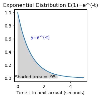
Example 2a) An exponential distribution has the form \(f(t)=ke^{-kt}\) (\(0\le t \le \infty\)) where the parameter \(k\) is such that the mean is \(1/k\). Suppose the time to the next car arriving at the drive-thru is given by E(1) (i.e. k=1 so the mean is 1 minute). What is the probability that the next arrival is within 3 minutes?
Solution. probability = \(\int_0^3 e^{-t}\,dt= - e^{-t}\mid_0^3= -e^{-3}+e^0=1-e^{-3}\approx .95.\)
Show code cell source
import numpy as np
import matplotlib.pyplot as plt
f= lambda t: np.exp(-t)
x=np.linspace(0,5,100)
y=f(x)
plt.figure(figsize=(3,3))
plt.plot(x,y)
x1=np.linspace(0,3,10)
y1=f(x1)
plt.fill_between(x1,y1,color='lightgray')
plt.title('Exponential Distribution E(1)=e^(-t)')
plt.text(-.2,0,'Shaded area = .95')
plt.text(1,.6,'y=e^(-t)',color='b')
plt.xlabel('Time t to next arrival (seconds)')
Text(0.5, 0, 'Time t to next arrival (seconds)')
Example 2b) Find the value of \(k\) so that there is a 25% chance (probability=.25) that the next car will arrive within 1 minute.
Solution \(\int_0^1 k e^{-kt}\,dt = .25 \Rightarrow - e^{-kt}\mid_0^1=.25 \Rightarrow -e^{-k}+1=.25 \Rightarrow -e^{-k}=-.75\Rightarrow e^{-k}=.75.\) Take \(\ln()\) of both sides, we have \(-k=\ln(.75)\Rightarrow k=-\ln(.75)\approx .29.\)
Example 3a) Using the value of \(k\) given in 2b), find the probability \(F(x)\) that the next car will arrive within \(x\) minutes.
Solution \(F(x)=\int_0^x .29 e^{-.29t}\,dt= -e^{-.29t}\mid_0^x = -e^{-.29x}+1.\) That is \(F(x)=1-e^{-.29x}\)
Example 3b) Use your function in part a) to find the probability that the next car will arrive within 2 minutes.
Solution
\(F(2)=1-e^{-.29(2)}=1-e^{-.58}\approx .44\)
7.8.3. Use of Random Numbers#
We will explain how a value \(r\) generated by a PRNG (pseudo-random number generator) can be converted into values of random variables such as
A=length of time before the next car arrives at the parking lot
O=length of time to place an order
P=length of time to pay for the food
F=length of time to pick up food
A=Length of time before next arrival#
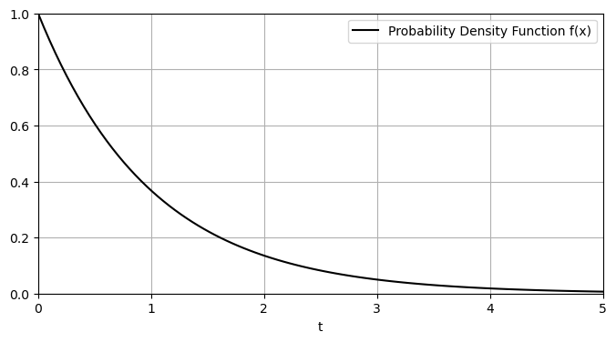
Let \(X\) be a random variable giving the length of time (in minutes) until the next car arrives at the parking lot. We assume \(X\) is an exponential distribution with mean \(1/k=1\). In this case, the probability density function (pdf) is
Show code cell source
import numpy as np
import matplotlib.pyplot as plt
x = np.linspace(0,5,100)
f= np.exp(-x)  #standard (unit) normal distribution
plt.figure(figsize=(8, 4))
plt.plot(x,f,color='k',label="Probability Density Function f(x)")
plt.xlim((0,5))
plt.ylim((0,1))
plt.xlabel("t")
plt.grid()
plt.legend()
plt.show()
The corresponding cumulative distribution function (cdf) is
Here is a graph of this cdf:
Show code cell source
import numpy as np
import matplotlib.pyplot as plt
t = np.linspace(0,5,100)
F= 1-np.exp(-t)  #standard (unit) normal distribution
plt.figure(figsize=(8, 4))
plt.plot(t,F,color='k',label="Cumulative Distribution F(t)")
plt.xlim((0,5))
plt.ylim((0,1))
plt.xlabel("A=time to next arrival (in minutes)")
plt.grid()
plt.legend()
plt.show()
Note that the \(F(t)=1-e^{-t}\) is an increasing function with a value of 0 at \(t=0\) and a range \([0,1)\). As such, each random number \(r\) \((0\le r <1)\) corresponds to a unique value of \(A\):
Show code cell source
import numpy as np
import matplotlib.pyplot as plt
t = np.linspace(0,5,100)
F= 1-np.exp(-t)  #standard (unit) normal distribution
plt.figure(figsize=(8, 4))
plt.plot(t,F,color='k',label="Cumulative Distribution F(t)")
plt.xlim((0,5))
plt.ylim((0,1))
plt.text(-.15,.7,"r",color='r',size=15)
plt.text(-np.log(1-.7)-.07,-.05,"A=-ln(1-r)",color='r',size=15)
plt.plot([0,-np.log(.3),-np.log(.3)],[.7,.7,0],color='r')
plt.xlabel("A=time to next arrival (in minutes)")
plt.grid()
plt.legend()
plt.show()
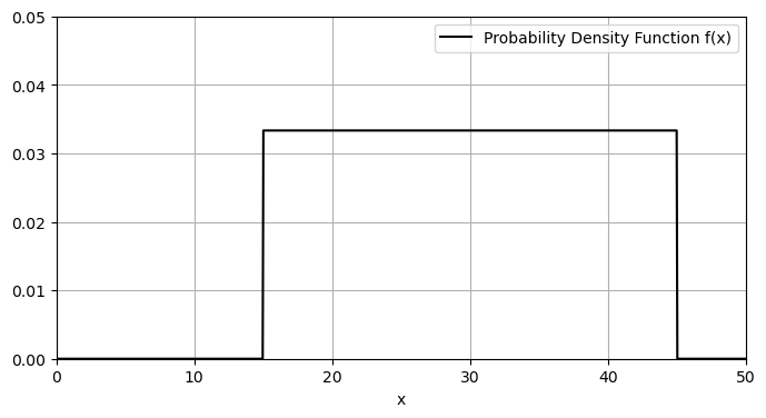
O=length of time to place an order#
Let \(X\) be a random variable giving the length of time (in seconds) to place an order. We assume \(X\) is uniformly distributed on the interval [15,45] (denoted U(15,45)) In this case, the probability density function (pdf) is
Show code cell source
import numpy as np
import matplotlib.pyplot as plt
x = np.linspace(0,50,1000)
f= (1/30)*(np.heaviside(x-15,0)-np.heaviside(x-45,0))   #standard (unit) normal distribution
plt.figure(figsize=(8, 4))
plt.plot(x,f,color='k',label="Probability Density Function f(x)")
plt.xlim((0,50))
plt.ylim((0,.05))
plt.xlabel("x")
plt.grid()
plt.legend()
plt.show()
Then, the cumulative distribution function (cdf) is
Here is a graph of this cdf:
Show code cell source
import numpy as np
import matplotlib.pyplot as plt
t = np.linspace(15,45,100)
F= ((t-15)/30)*np.heaviside(t-15,0)  #U(30,15)
plt.figure(figsize=(8, 4))
plt.plot(t,F,color='k',label="Cumulative Distribution F(t)")
plt.xlim((15,45))
plt.ylim((0,1))
plt.xlabel("O=time to place order (in seconds)")
plt.grid()
plt.legend()
plt.show()
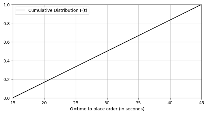
As before, the \(F(t)=\frac{t-15}{30}\) \(\,(15 \le t \le 45\)) is an increasing function with a value of 0 at \(t=15\) and a range \([0,1)\).
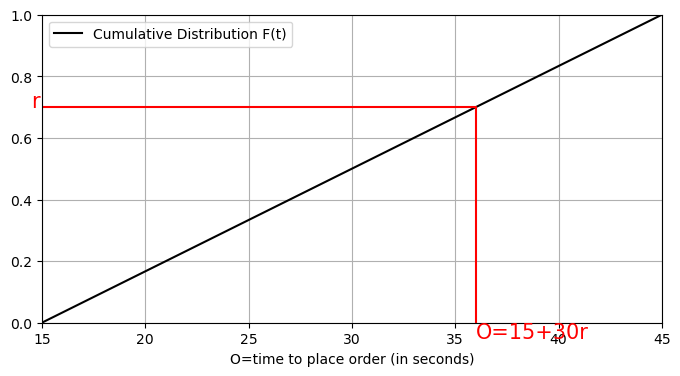
As such, each random number \(r\) \((0\le r <1)\) corresponds to a unique value of \(O\) where \(\,15 \le O\le 45\):
Show code cell source
import numpy as np
import matplotlib.pyplot as plt
t = np.linspace(15,45,100)
F= ((t-15)/30)*np.heaviside(t-15,0) # U(30,15)
plt.figure(figsize=(8, 4))
plt.plot(t,F,color='k',label="Cumulative Distribution F(t)")
plt.xlim((15,45))
plt.ylim((0,1))
plt.text(15-.5,.7,"r",color='r',size=15)
plt.text(15+30*.7,-.05,"O=15+30r",color='r',size=15)
plt.plot([15,15+30*.7,15+30*.7],[.7,.7,0],color='r')
plt.xlabel("O=time to place order (in seconds)")
plt.grid()
plt.legend()
plt.show()
7.8.4. Exercises#
Exercises
An important probability function called the exponential distribution has the form
The exponential distribution is used to describe the amount of time until some event occurs such as the time to the next arrival of a car at a drive-thru window. More specifically, the probability that the next car arrives somewhere between \(t=a\) and \(t=b\) minutes is given by the definite integral
a) Suppose \(k=1\). Find the probability that the next car will arrive at the drive-thru within 2 minutes.
b) Using \(k=1\), show that the probability that the next car will arrive between 0 and \(\infty\) minutes is equal to 1 (i.e. there is a 100% chance another car will arrive sometime in the future).
c) Find the value of \(k\) such that there is a 50% chance (i.e. probability = .5) that the next car will arrive in one minute.
d) Using your answer to part c), find a function \(F(x)\) which gives the probability that the next car will arrive within \(x\) minutes. (In general, given a probability distribution function \(f(t)\) defined on an interval \(a\le x \le b\), the cumulative distribution function \(F(x)\) is obtained by the definite integral \(\int_a^x f(t) \hspace{.1in} dt\)).
e) Use your answer to d) to find the probability that the next car will arrive within 3 minutes.
Let \(P=\) length of time to pay for an order of food.
a) Let \(X\) be a random variable giving the length of time (in seconds) to pay for an order using cash. We assume \(X\) is uniformly distributed on the interval [5,35] (denoted U(5,35)). Explain how to use a pseudo-random number to give a value for \(P\).
b) Let \(X\) be a random variable giving the length of time (in seconds) to pay for an order using a credit card. We assume \(X\) is uniformly distributed on the interval [5,20] (denoted U(5,20)). Explain how to use a pseudo-random number to give a value for \(P\).
Let \(F\) be the length of time to pick up food. Let \(X\) be a random variable giving the length of time (in seconds) to pick up an order. We assume \(X\) is uniformly distributed on the interval [30,90] (denoted U(30,90). Show how to use a pseudo-random number to generate a value for \(F\)