9.7. Solutions to Exercises#
SECTION 9.2.2 Linear Systems
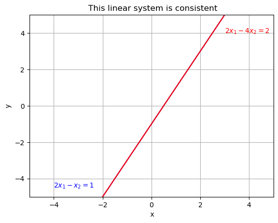
Find a linear system containing two equations in two unknowns that have infinitely many solutions. Verify your answer by plotting the lines of these equations on the same plane.
Solution:
The following system is consistent and has infinitely many solutions:
We expect that the graph of these two lines will coincide. Let’s plot the graph of these lines on the same plane:
import matplotlib.pyplot as plt
import numpy as np

# Data for plotting

x = range(-5, 5)
y1 = [ 2*k-1 for k in x]
y2 = [ 2*k-1 for k in x]

fig, ax = plt.subplots()

# Specify the length of each axis
ax.set_xlim(-5,5)
ax.set_ylim(-5,5)

#Plot x and y1 using blue color
ax.plot(x, y1, color = 'b')
ax.text(-4,-4.5,'$2x_1 - x_2 = 1$', color = 'b')

#Plot x and y2 using red color
ax.plot(x, y2, color = 'r')
ax.text(3,4,'$2x_1 -4x_2 = 2$', color = 'r')


# Add labels and a title to the graph
ax.set(xlabel=' x', ylabel='y',
       title=' This linear system is consistent')
ax.grid()

plt.show()
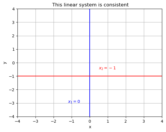
Find a linear system that is equivalent to the linear system in Example 1.
Solution:
Any system that has the same solution set as the linear system in Example 1 is considered equivalent. Since the solution set is \(\{(0, -1)\}\), the following system is an example of such a system:
# Data for plotting

r = range(-5, 5)
x1 = [ 0 for k in r]
y1 = [-1 for k in r]

fig, ax = plt.subplots()

# Specify the length of each axis
ax.set_xlim(-4,4)
ax.set_ylim(-4,4)

#Plot x and y1 using blue color
ax.plot(x1, r, color = 'b')
ax.text(-1.2,-3,'$x_1 = 0$', color = 'b')

#Plot x and y2 using red color
ax.plot(x, y1, color = 'r')
ax.text(0.5,-0.5, '$x_2 = -1$', color = 'r')


# Add labels and a title to the graph
ax.set(xlabel=' x', ylabel='y',
       title=' This linear system is consistent')
ax.grid()

plt.show()
Determine which of the following matrices are in REF. For those that are, identify their pivot columns. Are there any in RREF?
\(A = \begin{bmatrix} 0 & 0 & 4 &-1 && 0\\ 0 & 0 & 0 &0 && 0 \\ 0 & 0& 0 & 0 &&3\end{bmatrix}\)
\(B = \begin{bmatrix} 1 & 1 & 0 && 1\\ 0 & 1 & 1 &&0\\ 0 & 0 & 1 &&1 \end{bmatrix}\)
\(C = \begin{bmatrix} 1 & 0 & 3 && 0\\ 0 & 1 & 0 &&0\\ 0 & 0 & 0 &&1 \end{bmatrix}\)
\(D = \begin{bmatrix} 0 & 1 & 2\\ 1 & 0 & 3\\ 4 & -3 & 8 \end{bmatrix}\)
A matrix is in row echelon form (REF) if it satisfies the following conditions:
The rows with all zeros must be at the bottom.
Every leading term of a row must be in a column to the right of the leading entry.
Entries below a leading entry must be zero.
Let’s analyze each matrix and determine if they are in REF:
Matrix A is not in REF because it does not satisfy the first condition (rows with all zeros must be at the bottom).
Matrix B is in REF as it satisfies all the conditions.
Matrix C is in REF as it satisfies all the conditions.
None of the matrices A, B, or C are in reduced row echelon form (RREF) because the conditions for RREF include having a pivot of 1 in every row, and both matrix A and matrix C have nonzero pivots other than 1.
For the above matrices, write the corresponding linear systems and find their solutions.
Solution:
\(A:\)
Clearly, because of the last equation, this system is inconsistent.
\(B:\)
By back substitution, we can see that \( x_1 = 2 , -x_2 = x_3 = 1\).
\(C:\)
Clearly, because of the last equation, this system is inconsistent.
Find the REF of \(D = \begin{bmatrix} 0 & 1 & 2\\ 1 & 0 & 3\\ 4 & -3 & 8 \end{bmatrix}\).
Solution
D = np.array([[0,1,2],[1,0,3],[4,-3,8]])

# Elementry row operations:

# Swap two rows

def swap(matrix, row1, row2):

    copy_matrix=np.copy(matrix).astype('float64')

    copy_matrix[row1,:] = matrix[row2,:]
    copy_matrix[row2,:] = matrix[row1,:]

    return copy_matrix


# Multiple all entries in a row by a nonzero number


def scale(matrix, row, scalar):
    copy_matrix=np.copy(matrix).astype('float64')
    copy_matrix[row,:] = scalar*matrix[row,:]
    return copy_matrix

# Replacing a row by the sum of itself and a multiple of another

def replace(matrix, row1, row2, scalar):
    copy_matrix=np.copy(matrix).astype('float64')
    copy_matrix[row1] = matrix[row1]+ scalar * matrix[row2]
    return copy_matrix
D1 = swap(D, 0, 1)
D1
array([[ 1.,  0.,  3.],
       [ 0.,  1.,  2.],
       [ 4., -3.,  8.]])
D2 = replace(D1, 2, 0, -4)
D2
array([[ 1.,  0.,  3.],
       [ 0.,  1.,  2.],
       [ 0., -3., -4.]])
D3 = replace(D2, 2, 1, 3)
D3
array([[1., 0., 3.],
       [0., 1., 2.],
       [0., 0., 2.]])
SECTION 9.2.3 Matrix Equations
Given the system of equations:
Write this system as:
a vector equation.
a matrix equation.
Solution:
-Vector Equation:
-Matrix Equation:
True or False?
(a). \(\vec{0} \in \text{span} \{\vec{v}_1, \vec{v}_2, \vec{v}_3\}\).
(b). \(\vec{v}_1 \in \text{span} \{\vec{v}_1, \vec{v}_2, \vec{v}_3\}\).
(c). \(\text{span} \{\vec{v}_1, \vec{v}_2\} \subseteq \text{span} \{\vec{v}_1, \vec{v}_2, \vec{v}_3\}\).
(d). A set 4 vectors must be linearly DEPENDENT in \(\mathbb{R}^3\).
Solution:
(a)
True. The zero vector is always in the span of any set of vectors. This is because the span of a set of vectors includes all possible linear combinations of those vectors, and
is a linear combination of \(\vec{v_1}, \vec{v_2}\) and \(\vec{v_3}\).
(b)
\(\vec{v}_1 \in \text{span} \{\vec{v}_1, \vec{v}_2, \vec{v}_3\}\):
True. Since \(\vec{v}_1\) is a linear combination of \(\vec{v}_1, \vec{v}_2\) and \(\vec{v}_3\}\):
(c)
\(\text{span} \{\vec{v}_1, \vec{v}_2\} \subseteq \text{span} \{\vec{v}_1, \vec{v}_2, \vec{v}_3\}\):
True. Any linear combination of \(\vec{v}_1\) and \(\vec{v}_2\) is also a linear combination of \(\vec{v}_1\), \(\vec{v}_2\), and \(\vec{v}_3\):
(d)
A set of 4 vectors must be linearly dependent in \(\mathbb{R}^3\):
True. If we use the four vectors as columns of a matrix \(A\), then \(A\) will be \(3 \times 4\) which cannot have a pivot in every column. So the homogeneous system \(A\vec{x}= 0\) has nontrivial solutions making the columns DEPENDENT.
SECTION 9.2.4 Solution Set of Linear Systems
Is
linearly independent or dependent?
Solution:
Let’s denote the given vectors as:
Now, we’ll set up the following linear combination and solve for the coefficients:
Substituting the given vectors and equating the resulting components to zero, we have the following linear system:
\(\{\vec{v_1}, \vec{v_2} \vec{v_3}\}\) is a linearly independent set is and only if this system has only the trivial solution. To verify this we set up the augmented matrix of this system and apply the row operations:
import numpy as np

A = np.array([[1, 4, 7, 0], [2, 5, 8, 0], [3, 6, 9, 0]])
A
array([[1, 4, 7, 0],
       [2, 5, 8, 0],
       [3, 6, 9, 0]])
A1 = replace(A, 1, 0, -2)
A1
array([[ 1.,  4.,  7.,  0.],
       [ 0., -3., -6.,  0.],
       [ 3.,  6.,  9.,  0.]])
A2 = replace(A1, 2, 0, -3)
A2
array([[  1.,   4.,   7.,   0.],
       [  0.,  -3.,  -6.,   0.],
       [  0.,  -6., -12.,   0.]])
A3 = replace(A2, 2, 1, -2)
A3
array([[ 1.,  4.,  7.,  0.],
       [ 0., -3., -6.,  0.],
       [ 0.,  0.,  0.,  0.]])
A4 = scale(A3, 1, -1/3)
A4
array([[ 1.,  4.,  7.,  0.],
       [-0.,  1.,  2., -0.],
       [ 0.,  0.,  0.,  0.]])
From see this we can see that \(c_3\) is a free variable and the system has infinitely many solutions, and thus, \(\{\vec{v_1}, \vec{v_2} \vec{v_3}\}\) is linearly dependent.
Describe the solution set of \(A\vec{x}=\vec{b}\) where
Solution:
Ab = np.array([[1,4,7,1],[2,5,8,2],[3,6,9,3]])
Ab

# Swap two rows

def swap(matrix, row1, row2):

    copy_matrix=np.copy(matrix).astype('float64')

    copy_matrix[row1,:] = matrix[row2,:]
    copy_matrix[row2,:] = matrix[row1,:]

    return copy_matrix


# Multiple all entries in a row by a nonzero number


def scale(matrix, row, scalar):
    copy_matrix=np.copy(matrix).astype('float64')
    copy_matrix[row,:] = scalar*matrix[row,:]
    return copy_matrix

# Replacing a row1 by the sum of itself and a multiple of row2

def replace(matrix, row1, row2, scalar):
    copy_matrix=np.copy(matrix).astype('float64')
    copy_matrix[row1] = matrix[row1]+ scalar * matrix[row2]
    return copy_matrix
B1 = replace(Ab, 1 , 0, -2)
B1
array([[ 1.,  4.,  7.,  1.],
       [ 0., -3., -6.,  0.],
       [ 3.,  6.,  9.,  3.]])
B2 = replace(B1, 2 , 0, -3)
B2
array([[  1.,   4.,   7.,   1.],
       [  0.,  -3.,  -6.,   0.],
       [  0.,  -6., -12.,   0.]])
B3 = replace(B2, 2, 1 , -2)
B3
array([[ 1.,  4.,  7.,  1.],
       [ 0., -3., -6.,  0.],
       [ 0.,  0.,  0.,  0.]])
B4 = scale(B3, 1 , -1/3)
B4
array([[ 1.,  4.,  7.,  1.],
       [-0.,  1.,  2., -0.],
       [ 0.,  0.,  0.,  0.]])
From this we see that for any \(z \in \mathbb{R}\) we have a unique solution. A general solution for this system is:
SECTION 9.3.1 Matrix Algebra
Which pair of the following matrices can be multiplied? Compute their matrix product.
\(A = \begin{bmatrix} 1 & 3 \\ 4 & -2 \\ 3 & 2 \end{bmatrix}\)
\(B = \begin{bmatrix} 1 & 4 & 5\\ 0 & 2 & 3 \end{bmatrix}\)
\(C = \begin{bmatrix} 1 & 3 & 0\\ 2 & -1 & 3 \\ 0 & 1 & 1 \end{bmatrix}\)
Solution:
import numpy as np

A = np.array([[1,3], [4,-2], [3,2]])

B = np.array([[1,4,5], [0,2,3]])

C = np.array([[1,3,0], [2,-1, 3], [0,1,1]])
None of \(AA\), \(CB\), \(BB\), and \(AC\) can be performed because none of the neighboring dimensions match. For example, if we try to compute \(AA\) in Python we get the following error:
A@A
---------------------------------------------------------------------------
ValueError                                Traceback (most recent call last)
Cell In[5], line 1
----> 1 A@A

ValueError: matmul: Input operand 1 has a mismatch in its core dimension 0, with gufunc signature (n?,k),(k,m?)->(n?,m?) (size 3 is different from 2)
On the other hand \(AB\), \(BC\), \(CA\), \(BA\), \(CC\) can be performed:
A@B
array([[ 1, 10, 14],
       [ 4, 12, 14],
       [ 3, 16, 21]])
B@C
array([[ 9,  4, 17],
       [ 4,  1,  9]])
C@A
array([[13, -3],
       [ 7, 14],
       [ 7,  0]])
C@C
array([[ 7,  0,  9],
       [ 0, 10,  0],
       [ 2,  0,  4]])
Find two matrices \(A\) and \(B\) such that the products \(AB\) and \(BA\) are defined but \(AB \neq BA\).
Solution:
A = np.array([[1, 2, 3], [4, 5, 6]])
B = np.array([[7, 8], [9, 10], [11, 12]])

AB = A@B
BA = B@A

print('AB = \n', AB)

print('\nBA = \n', BA)
AB =
 [[ 58  64]
 [139 154]]

BA =
 [[ 39  54  69]
 [ 49  68  87]
 [ 59  82 105]]
Given \(A= \begin{bmatrix} 1 & 2 \\ 1& 2 \end{bmatrix}\), find a nonzero matrix \(C\) for which \(AC= \begin{bmatrix} 0 & 0 \\ 0 & 0 \end{bmatrix}\).
Solution
There are infinitely many matrices such that \(AC = 0\). We can set \(C = \begin{bmatrix} c_1 & C_2 \\ C_3 & C_4 \end{bmatrix}\) and solve \(AC=0\) for C. For example one solution is \(C = \begin{bmatrix} -2 & 1 \\ 1 & 0.5 \end{bmatrix}\)
A = np.array([[1,2], [1,2]])

C = np.array([[-2,1], [1, -0.5]])


A@C
array([[0., 0.],
       [0., 0.]])
SECTION 9.3.2 Transpose, Inverse and Trace of matrices
Suppose \(A= \begin{bmatrix} 1 & 2 \\ 0 & -1 \\ 3 & 0 \end{bmatrix}\)
(a) Compute \(A^T\).
(b) Is \(AA^T\) invertible?
(c) Is \(A^TA\) invertible?
Solution:
# part(a)

A = np.array([[1,2], [0,-1], [3,0]])

# compute transpose of A
A_T = np.transpose(A)

A_T
array([[ 1,  0,  3],
       [ 2, -1,  0]])
(b)
Solution 1 Obviously a \(3\times 2\) matrix has at most two linearly independent columns. It can be shown that \(AA^T\) has the same amount of linearly independent columns. Thus \(AA^T\) as a \(3\times 3\) matrix does not have three linearly independent columns and therefore, is not invertible by the invertible matrix theorem.
Solution 2 Lets check and see if \(AA^T\) row equivalent to identity matrix \(I_3\)
# part(b)

B = A @ A_T
B
array([[ 5, -2,  3],
       [-2,  1,  0],
       [ 3,  0,  9]])
We form the augmented matrix \([AA^T\ |\ I_3]\) and use row operations to check if it is invertible:
# 3x3 Identity matrix
I3 = np.eye(3)

# Augmented matrix [AA^T, I_3]
M = np.concatenate((B, I3), axis=1)
M
array([[ 5., -2.,  3.,  1.,  0.,  0.],
       [-2.,  1.,  0.,  0.,  1.,  0.],
       [ 3.,  0.,  9.,  0.,  0.,  1.]])
We can now use the following row operations to check if \(B\) is row equivalent to the identity matrix.
# Swap two rows

def swap(matrix, row1, row2):

    copy_matrix=np.copy(matrix).astype('float64')

    copy_matrix[row1,:] = matrix[row2,:]
    copy_matrix[row2,:] = matrix[row1,:]

    return copy_matrix


# Multiple all entries in a row by a nonzero number


def scale(matrix, row, scalar):
    copy_matrix=np.copy(matrix).astype('float64')
    copy_matrix[row,:] = scalar*matrix[row,:]
    return copy_matrix

# Replacing row1 by the sum of itself and a multiple of row2

def replace(matrix, row1, row2, scalar):
    copy_matrix=np.copy(matrix).astype('float64')
    copy_matrix[row1] = matrix[row1]+ scalar * matrix[row2]
    return copy_matrix
M1 = swap(M, 0, 1)
M1
array([[-2.,  1.,  0.,  0.,  1.,  0.],
       [ 5., -2.,  3.,  1.,  0.,  0.],
       [ 3.,  0.,  9.,  0.,  0.,  1.]])
M2 = scale(M1, 0, -1/2)
M2
array([[ 1. , -0.5, -0. , -0. , -0.5, -0. ],
       [ 5. , -2. ,  3. ,  1. ,  0. ,  0. ],
       [ 3. ,  0. ,  9. ,  0. ,  0. ,  1. ]])
M3 = replace(M2, 1, 0, -5)
M3
array([[ 1. , -0.5, -0. , -0. , -0.5, -0. ],
       [ 0. ,  0.5,  3. ,  1. ,  2.5,  0. ],
       [ 3. ,  0. ,  9. ,  0. ,  0. ,  1. ]])
M4 = replace(M3, 2, 0, -3)
M4
array([[ 1. , -0.5, -0. , -0. , -0.5, -0. ],
       [ 0. ,  0.5,  3. ,  1. ,  2.5,  0. ],
       [ 0. ,  1.5,  9. ,  0. ,  1.5,  1. ]])
M5 = scale(M4, 1, 2)
M5
array([[ 1. , -0.5, -0. , -0. , -0.5, -0. ],
       [ 0. ,  1. ,  6. ,  2. ,  5. ,  0. ],
       [ 0. ,  1.5,  9. ,  0. ,  1.5,  1. ]])
M6 = replace(M5, 2, 1, -1.5)
M6
array([[ 1. , -0.5, -0. , -0. , -0.5, -0. ],
       [ 0. ,  1. ,  6. ,  2. ,  5. ,  0. ],
       [ 0. ,  0. ,  0. , -3. , -6. ,  1. ]])
From this we can see that it is impossible to get an identity matrix on the left side, so \(AA^T\) is not invertible.
(C):
Let’s compute \(A^TA\)
C = A_T @ A
C
array([[10,  2],
       [ 2,  5]])
The determinant of \(C\) is \(50 - 4 = 46\), not zero, and therefore, \(C\) is invertible.
The trace is invariant under cyclic permutations, i.e., for three matrices we have \(Tr(ABC) = Tr(BCA) = Tr(CAB)\), where \(A\) is an \(n\times p\) matrix, \(B\) is a \(p\times m\) matrix, and \(C\) is an \(m \times n\) matrix.
Using Example 9, generate three matrices \(A\), \(B\), and \(C\) such that the product \(ABC\) makes sense, and verify that:
Solution
# generate a 5x3 matrix
A = np.random.rand(5, 3)

# generate a 3x2 matrix
B = np.random.rand(3, 2)


# generate a 2x5 matrix
C = np.random.rand(2, 5)

# find ABC
ABC = A @ B @ C

print('ABC = \n \n ', ABC)

# find BCA

BCA = B @ C @ A

print('\n BCA = \n \n ', BCA)

# find CAB

CAB = C @ A @ B

print('\n CAB = \n \n ', CAB)

#trace of ABC

Tr_ABC = np.trace(ABC)
print('\n Tr(ABC) = ', Tr_ABC)

Tr_BCA = np.trace(BCA)
print('\n Tr(BCA) = ', Tr_BCA)

Tr_CAB = np.trace(CAB)
print('\n Tr(CAB) = ', Tr_CAB)
ABC =

  [[0.98987463 1.14173923 0.9749678  0.54548799 1.17771615]
 [0.68823143 0.79423646 0.62002792 0.3285909  0.78062694]
 [0.89061397 1.02686076 0.93109763 0.53800509 1.09521993]
 [1.01585235 1.17163085 1.01045759 0.56847944 1.21516502]
 [1.32387689 1.52734839 1.25343552 0.68530018 1.54173913]]

 BCA =

  [[1.20700173 1.31688659 1.02761727]
 [2.75843882 3.01690466 2.4760114 ]
 [0.59342757 0.65299393 0.60152091]]

 CAB =

  [[2.1970437  2.34545965]
 [2.3243565  2.6283836 ]]

 Tr(ABC) =  4.825427299545087

 Tr(BCA) =  4.825427299545087

 Tr(CAB) =  4.825427299545087
SECTION 9.3.3 Determinant
Let \(A\) be an \(n\times n\) matrix such that \(A^2 = I_n\). Show that \(det(A) = \pm 1\).
Solution:
By Theorem 4, part (2), \(\text{det}(AA) = \text{det}(A) \cdot \text{det}(A) = \text{det}(A)^{2}\). Theorem 1, we have \(\text{det}(I_n) = 1\). Therefore,
Which means
Find the determinant of \(A = \begin{bmatrix} 1 & 1 & 2 \\ 2 & 0 & 3 \\ 5 & -3 & 8 \end{bmatrix}\) using the row reduction method. Is \(A\) invertible?
Solution:
A = np.array([[1,1,2], [2,0,3], [5,-3,8]])

# Elementry row operations:

# Swap two rows

def swap(matrix, row1, row2):

    copy_matrix=np.copy(matrix).astype('float64')

    copy_matrix[row1,:] = matrix[row2,:]
    copy_matrix[row2,:] = matrix[row1,:]

    return copy_matrix


# Multiply all entries in a row by a nonzero number


def scale(matrix, row, scalar):
    copy_matrix=np.copy(matrix).astype('float64')
    copy_matrix[row,:] = scalar*matrix[row,:]
    return copy_matrix

# Replacing a row1 by the sum of itself and a multiple of row2

def replace(matrix, row1, row2, scalar):
    copy_matrix=np.copy(matrix).astype('float64')
    copy_matrix[row1] = matrix[row1]+ scalar * matrix[row2]
    return copy_matrix
A
array([[ 1,  1,  2],
       [ 2,  0,  3],
       [ 5, -3,  8]])
A1 = replace(A, 1, 0, -2)
A1
array([[ 1.,  1.,  2.],
       [ 0., -2., -1.],
       [ 5., -3.,  8.]])
A2 = replace(A1, 2, 0, -5)
A2
array([[ 1.,  1.,  2.],
       [ 0., -2., -1.],
       [ 0., -8., -2.]])
A3 = replace(A2, 2, 1, -4)
A3
array([[ 1.,  1.,  2.],
       [ 0., -2., -1.],
       [ 0.,  0.,  2.]])
\(A_3\) is already an upper-triangular matrix and we have
Since we haven’t used any swap operations we get:
Use determinants to decide if the set \(\left\lbrace \begin{bmatrix} 1 \\ 2 \\ 3 \end{bmatrix}, \begin{bmatrix} 4 \\ 5 \\ 6 \end{bmatrix}, \begin{bmatrix} 7 \\ 8 \\ 9 \end{bmatrix} \right\rbrace\) is linearly independent.
Solution:
A matrix A is invertible if and only if \(\text{det}(A)\neq 0\) (Theorem 3). By the invertible matrix theorem, we know that A is invertible if and only if the columns of A are linearly independent.
# matrix A
A = np.array([[1,4, 7], [2,5,8], [3,6,9]])


# Compute a 2x2 determinant
def det2(matrix):

    if matrix.shape == (2, 2):
        return matrix[0,0] * matrix[1,1] - matrix[0,1] * matrix[1,0]
    else:
        print("Please enter a 2x2 matrix")

# Computes the determinant of an n x n matrix.
def det(matrix):
    n = matrix.shape[0]
    if n == 1:
        return matrix[0, 0]
    elif n == 2:
        return matrix[0, 0] * matrix[1, 1] - matrix[0, 1] * matrix[1, 0]
    else:
        det = 0
        for j in range(n):
            submatrix = np.delete( (np.delete(matrix, 0 , 0)), j ,1)
            det += (-1) ** (0 + j) * matrix[0, j] * det2(submatrix)
        return det

print('det(A) = ', det(A))
det(A) = 0
Suppose \(A\), \(B\), \(P\) are \(n\times n\) matrices, \(P\) is invertible, and \(r\) is a real number. Mark True or False:
a. \(det(A+B) = det(A) + det(B)\).
b. \(det(rA) = r \cdot det(A)\).
c. \(det(PAP^{-1}) = det(A)\).
Solution
a. False. For example, consider matrices:
Clearly, \(\text{det}(A) = 2\), \(\text{det}(B) = 3\), and \(\text{det}(A+B) = 10\).
b. False. For example, let \(A = \begin{bmatrix} 1 & 0 \\ 0 & 2 \end{bmatrix}\) and \(r = 2\). Then, \(\text{det}(2A) = 8\), whereas \(2\text{det}(A) = 4\).
c. True. Using the invertibility of \(P\) and the properties of determinants, we have
Determine if the following points are coplanar (i.e., they lie on the same plane):
\[\begin{split}\begin{bmatrix} 1 \\ 0 \\ 2 \end{bmatrix}, \begin{bmatrix} 4 \\ 3 \\ 5 \end{bmatrix}, \begin{bmatrix} 3 \\ 0 \\ 6 \end{bmatrix}\end{split}\]
Solution:
A = np.array([[1,4,3], [0,3,0], [2,5,6]])
A
array([[1, 4, 3],
       [0, 3, 0],
       [2, 5, 6]])
print('det(A) = ', det(A))
det(A) = 0
SECTION 9.4.1 Subspaces of \(\mathbb{R}^n\)
Determine which one of the following sets is a subspace:
a. \(H = \left\lbrace \ \begin{bmatrix} x \\ y \\ z \end{bmatrix} \in \mathbb{R}^3 \mbox{ with } x \geq 0, \right\rbrace.\)
b. \(H = \left\lbrace \ \begin{bmatrix} x \\ 1 \\2x \end{bmatrix} \in \mathbb{R}^3 \right\rbrace.\)
Solution
a. is not a subspace because it is not closed under addition. For example, let
Then \(\vec{u}+ \vec{v}\) is not in \(H\).
b. \(H\) is not a subspace because \(\vec{o}\) is not in \(H\).
Let \(A = \begin{bmatrix} 1 & 2 &-9 \\ -2 & -2 & 2 \\ 2 & 3 &0 \end{bmatrix}\). Find a basis for \(col(A)\) and \(null(A)\).
Solution:
We use row operation to find the pivot columns of \(A\):
import numpy as np

A = np.array([[1,2,-9], [-2,-2,2],[2,3,0]])

# Elementry row operations:

# Swap two rows

def swap(matrix, row1, row2):

    copy_matrix=np.copy(matrix).astype('float64')

    copy_matrix[row1,:] = matrix[row2,:]
    copy_matrix[row2,:] = matrix[row1,:]

    return copy_matrix


# Multiply all entries in a row by a nonzero number


def scale(matrix, row, scalar):
    copy_matrix=np.copy(matrix).astype('float64')
    copy_matrix[row,:] = scalar*matrix[row,:]
    return copy_matrix

# Replacing a row1 by the sum of itself and a multiple of row2

def replace(matrix, row1, row2, scalar):
    copy_matrix=np.copy(matrix).astype('float64')
    copy_matrix[row1] = matrix[row1]+ scalar * matrix[row2]
    return copy_matrix
A
array([[ 1,  2, -9],
       [-2, -2,  2],
       [ 2,  3,  0]])
A1 = replace(A, 1, 0, 2)
A1
array([[  1.,   2.,  -9.],
       [  0.,   2., -16.],
       [  2.,   3.,   0.]])
A2 = replace(A1, 2, 0, -2)
A2
array([[  1.,   2.,  -9.],
       [  0.,   2., -16.],
       [  0.,  -1.,  18.]])
A3 = scale(A2, 1, 0.5)
A3
array([[ 1.,  2., -9.],
       [ 0.,  1., -8.],
       [ 0., -1., 18.]])
A4 = replace(A3, 2, 1, 1)
A4
array([[ 1.,  2., -9.],
       [ 0.,  1., -8.],
       [ 0.,  0., 10.]])
From this we can see that all columns are pivots and the columns of \(A\) form a basis for \(\text{col}(A)\):
Therefore, \(dim(\text{col}(A) = 3)\). By Rank-Nulity Theorem, \(dim(\text{null}(A) = 0)\), or in other words, \(\text{null}(A) = \vec{o}\). We could also form the augmented matrix \([A|0]\) and find the RREF of it:
# zero vector
O = np.array([np.zeros(3)]).T
O
array([[0.],
       [0.],
       [0.]])
# Augmented matrix [A|0]

B = np.concatenate((A, O) , axis = 1)
B
array([[ 1.,  2., -9.,  0.],
       [-2., -2.,  2.,  0.],
       [ 2.,  3.,  0.,  0.]])
B1 = replace(B, 1, 0 , 2)
B1
array([[  1.,   2.,  -9.,   0.],
       [  0.,   2., -16.,   0.],
       [  2.,   3.,   0.,   0.]])
B2 = replace(B1, 2, 0, -2)
B2
array([[  1.,   2.,  -9.,   0.],
       [  0.,   2., -16.,   0.],
       [  0.,  -1.,  18.,   0.]])
B3 = scale(B2, 1, 0.5)
B3
array([[ 1.,  2., -9.,  0.],
       [ 0.,  1., -8.,  0.],
       [ 0., -1., 18.,  0.]])
B4 = replace(B3, 2, 1, 1)
B4
array([[ 1.,  2., -9.,  0.],
       [ 0.,  1., -8.,  0.],
       [ 0.,  0., 10.,  0.]])
B5 = scale(B4, 2, 1/10)
B5
array([[ 1.,  2., -9.,  0.],
       [ 0.,  1., -8.,  0.],
       [ 0.,  0.,  1.,  0.]])
B6 = replace(B5, 0, 1, -2)
B6
array([[ 1.,  0.,  7.,  0.],
       [ 0.,  1., -8.,  0.],
       [ 0.,  0.,  1.,  0.]])
B7 = replace(B6, 0, 2, -7)
B7
array([[ 1.,  0.,  0.,  0.],
       [ 0.,  1., -8.,  0.],
       [ 0.,  0.,  1.,  0.]])
B8 = replace(B7, 1, 2, 8)
B8
array([[1., 0., 0., 0.],
       [0., 1., 0., 0.],
       [0., 0., 1., 0.]])
Suppose \(A\) is a \(5 \times 5\) matrix, and \(A\) has 3 pivot columns.
a. Prove that \(A\vec{x}=\vec{0}\) must have nontrivial solutions.
b. Is there an example of \(A\) where \(col(A)= null(A)\)?
Solution:
a. By Rank-Nullity Theorem, \(dim(\text{null}(A) = 2)\) so it is not trivial.
b. No, it is not because in such a matrix we would have
which is not possible.
Find an explicit example of a \(4\times 4\) matrix \(A\) which has \(colA = null(A)\)
Solution:
Let
Clearly, \(\vec{u} = \begin{bmatrix} 0 \\ 0 \\ 1 \\ 0 \end{bmatrix}\) and \(\vec{v} = \begin{bmatrix} 0 \\ 0 \\ 0 \\ 1 \end{bmatrix}\) form a basis for \(\text{col}(A)\). We can easily verify that \(A\vec{u} = A\vec{v} = \vec{0}\), indicating that \(\vec{u}\) and \(\vec{v}\) are in \(null(A)\). Now, we will show that they also form a basis for \(null(A)\).
According to the rank-nullity theorem, we know that \(\text{dim}(null(A)) = 2\). Thus, if we show that \(\vec{u}\) and \(\vec{v}\) are linearly independent, we are done! Fortunately, they are linearly independent because they are not multiples of each other.
SECTION 9.4.2 Introduction to Linear Transformations
Determine if each transformation is linear
a. \(T: \mathbb{R}^2 \rightarrow \mathbb{R}^2\) given by
b. \(H: \mathbb{R}^2 \rightarrow \mathbb{R}^2\) given by
Solution:
(a): \(T\) is a linear transformation since
and
(b) \(H\) is not a linear transformation because
but
Find the standard matrix of \(T: \mathbb{R}^2 \rightarrow \mathbb{R}^2\) given by \(T(\vec{x}) =\) first reflect \(\vec{x}\) across the \(x\)-axis and then rotate \(45^\circ\) counterclockwise.
Solution:
To find the standard matrix representation of \(T\) we apply \(T\) to the standard basis vectors of \(\mathbb{R}^2\):
\(T\) reflects \(\begin{bmatrix} 1 \\ 0 \end{bmatrix}\) to itself and then rotates it to \(\begin{bmatrix} \frac{\sqrt{2}}{2} \\ \frac{\sqrt{2}}{2} \end{bmatrix}\).
\(T\) reflects \(\begin{bmatrix} 0 \\ 1 \end{bmatrix}\) to \(\begin{bmatrix} 0 \\ -1 \end{bmatrix}\) and then rotates it to \(\begin{bmatrix} \frac{\sqrt{2}}{2} \\ -\frac{\sqrt{2}}{2} \end{bmatrix}\).
Therefore, the standard matrix of \(T\) is \(\begin{bmatrix} \frac{\sqrt{2}}{2} & \frac{\sqrt{2}}{2} \\ \frac{\sqrt{2}}{2} & - \frac{\sqrt{2}}{2} \end{bmatrix}\).
Suppose \(T: \mathbb{R}^2 \rightarrow \mathbb{R}^3\) is a linear map and
Find \(T \begin{bmatrix} 2 \\ 3 \end{bmatrix}\).
Solution
Note that
Now
9.5.3 Eigenspace and characteristic polynomial
If \(\vec{v}\) is an eigenvector of \(A\) corresponding to \(\lambda\),what is \(A^3\vec{v}\).
Solution:
If A is an \(n\times n\) matrix and \(2\) is an eigenvalue of \(A\), show that \(4\) is an eigenvalue of \(2A\).
Solution:
Let \(\vec{v}\) be an eigenvector of \(A\) corresponding to \(\lambda = 2\). We have:
If \(A\) is an invertible matrix with eigenvalue \(\lambda\) show that \(A^{-1}\) has eigenvalue \(1/\lambda.\)
Solution:
Let \(\vec{v}\) be an eigenvector of \(A\) corresponding to \(\lambda\). We have
Let \(A = \begin{bmatrix} 1 & 3 & 3\\ -3 & -5 &-3\\ 3 & 3 & 1 \end{bmatrix}\).
a. Find the eigenvalues of \(A\) and their multiplicities.
b. For each eigenvalue in part (a) find the corresponding eigenspace.
c. Find the dimension of each eigenspace in part (b) by finding a basis for it. How this result is related to your answer to part (a)?
Solution:
import numpy as np

#(a)

A = np.array([[1,3,3], [-3, -5, -3], [3,3,1]])

#eigenvalues of A
np.linalg.eigvals(A)
array([ 1., -2., -2.])
(b)
and
(c) A basis for \(E_1: \left\{ \ \begin{bmatrix} 1\\-1\\1 \end{bmatrix}\ \right\}\). The dimension of \(E_1\) is then \(1\).
A basis for \(E_{-2}: \left\{\ \begin{bmatrix} -1\\ 1 \\ 0 \end{bmatrix}, \begin{bmatrix} -1 \\ 0\\ 1 \end{bmatrix}\ \right\}\)
The dimension of \(E_{-2}\) is then \(2\).
The multiplicity of \(\lambda = 1\) is equal to the dimension of \(E_{1}\). The multiplicity of \(\lambda = -2\) is equal to the dimension of \(E_{-2}\).
In general the multiplicity of an eigenvalue \(\lambda\) is not equal to the dimension of its eigenspace \(E_{\lambda}\). However, when it does we say the matrix is diagonalizable. We will learn more about this in the next section.
SECTION 9.5.4 Diagonalization
Suppose \( M = \begin{bmatrix} 2 & 4 & 3 \\ -4 & -6 & -3 \\ 3 & 3 & 1 \end{bmatrix}. \)
a. Is M diagonalizable? If yes find a diagonalization for it.
b. Use this diagonalization to compute \(M^(100)\)
Solution:
(a)
M = np.array([[2,4,3], [-4,-6,3], [3,3,1]])
# find evalues and evectors
evalues, evectors = np.linalg.eig(M)

print("eigenvalues = ",  evalues)
eigenvalues = [-5. -2. 4.]
Since we have three distinct eigenvalues, \(M\) is diagonalizable.
lambda_1 = evalues[0]
lambda_2 = evalues[1]
lambda_3 = evalues[2]

# finding the diagonal matrix D
D = np.array([[lambda_1, 0, 0], [0, lambda_2, 0], [0, 0, lambda_3]])

# finding the invirtible matrix P
P = evectors

# finding the inverse of matrix P

Q = np.linalg.inv(P)

#sanity check: A = PDQ

P @ D @ Q
array([[ 2.,  4.,  3.],
       [-4., -6.,  3.],
       [ 3.,  3.,  1.]])
(b): Note that
# finding D^10

## digonal entries to the power of 10 (rounded it up to the closest intiger)
a1 = np.rint(pow(evalues[0], 100))
a2 = np.rint(pow(evalues[1], 100))
a3 = np.rint(pow(evalues[2], 100))

# computing D to the power of 10
D100 = np.array([[ a1, 0, 0], [0, a2, 0], [0, 0, a3]])

print(D100)

A100 = P @ D100 @ Q

A100
[[7.88860905e+69 0.00000000e+00 0.00000000e+00]
 [0.00000000e+00 1.26765060e+30 0.00000000e+00]
 [0.00000000e+00 0.00000000e+00 1.60693804e+60]]
array([[-4.38256058e+69, -4.38256058e+69,  4.38256059e+69],
       [ 9.64163329e+69,  9.64163329e+69, -9.64163329e+69],
       [-2.62953635e+69, -2.62953635e+69,  2.62953635e+69]])
Suppose \(C=\begin{bmatrix} 3 & 0 & 1 & 0 & 0\\ 0 & 3 & 0 & 0 & 0\\ 0 & 0 & 3 & 0 & 0\\ 0 & 0 & 3 & 2 & 0\\ 0 & 0 & 0 & 0 & 2 \end{bmatrix}\). Is \(C\) diagonalizable?
Solution:
No. The eigenvalues of \(C\) are 3 with multiplicity 3 and 2 with multiplicity 2. We show C is not diagonalizable by looking for the dimension of \(E_3 = Nul(C-3I).\)
C = np.array([[3,0,1, 0, 0], [0,3,0,0,0], [0,0,3,0,0], [0,0,3,2,0], [0,0,0,0,2]])

# find eigenvalues and eigenvectors
evalues, evectors = np.linalg.eig(C)

print('eigenvalues = ',evalues)

#identity matrix
I = np.eye(5)

# constructing C-3I
C - 3*I
eigenvalues = [3. 3. 2. 3. 2.]
array([[ 0.,  0.,  1.,  0.,  0.],
       [ 0.,  0.,  0.,  0.,  0.],
       [ 0.,  0.,  0.,  0.,  0.],
       [ 0.,  0.,  3., -1.,  0.],
       [ 0.,  0.,  0.,  0., -1.]])
From this, we can see that the number of non-pivot columns in \(E_3\) is 2 which is not equal to 3. Thus \(C\) is not diagonalizable.
Let \(A\) be a \(5\times 5\) matrix, with two eigenvalues. One eigenspace is three-dimensional, the other is two dimensional. Is \(A\) diagonalizable?
Solution:
Yes, since we have \(5\) linearly independent eigenvectors of \(A.\)
Compute \(A^{200}\) where \(A = \begin{bmatrix} 4 & -3\\ 2 & -1 \end{bmatrix}\).
Solution:
We can easily check that \(A\) has two distinct eigenvalues and therefore diagonalizable. Let’s find a diagonalization for it.
A = np.array([[1,2], [4,3]])

# find evalues and evectors
evalues, evectors = np.linalg.eig(A)

lambda_1 = evalues[0]
lambda_2 = evalues[1]

# finding the diagonal matrix D
D = np.array([[lambda_1, 0], [0, lambda_2]])

# finding the invirtible matrix P
P = evectors

# finding the inverse of matrix P

Q = np.linalg.inv(P)

#sanity check: A = PDQ

P @ D @ Q
array([[1., 2.],
       [4., 3.]])
# finding D^200

a1 = np.rint(pow(evalues[0], 200))
a2 = np.rint(pow(evalues[1], 200))

# computing D to the power of 20
D200 = np.array([[ a1, 0], [0, a2]])

# computing A to the power of 20

A200 = P @ D200 @ Q

A200
array([[2.07433843e+139, 2.07433843e+139],
       [4.14867685e+139, 4.14867685e+139]])
SECTION 9.5.5 Discrete Dynamical Systems
Let \(A\) be a \(2\times 2\) matrix with eigenvalues \(5\) and \(\frac{1}{5}\) and corresponding eigenvectors \(\begin{bmatrix} 1 \\ 1 \end{bmatrix}\) and \(\begin{bmatrix} -1 \\ 1 \end{bmatrix}\). Let \(\vec{x}_k\) be a solution of \(\vec{x}_{k+1} = A \vec{x}_{k}\), \(\vec{x}_0 = \begin{bmatrix} 9 \\ 1 \end{bmatrix}\) .
a. Compute \(\vec{x}_1 = A\vec{x}_0\)
b. Find a formula for \(\vec{x}_k\) involving \(k\) and the eigenvectors of \(A\).
c. Describe what happens when \(k\to \infty\).
Solution:
#(a)

# initial vector
x_0 = np.array([9,1])

# matrix A
A = np.array([[1,-1],[1,1]])

#x_1
x_1 = A @ x_0
x_1
array([ 8, 10])
(b)
Assume
Then
# a matrix whose columns are eigenvectors
P = np.array([[1,-1], [1,1]])

#solving (*) for coeeficients d1 and d2

D = np.linalg.solve(P, x_0)

print('d1 = ', D[0], ' and d2 = ',D[1] )
d1 = 5.0 and d2 = -4.0
Therefore, we have
(C)
SECTION 9.6.1 Inner product and Orthogonality
Let \( \vec{a} = \begin{bmatrix}1 \\ 2 \\ 3 \\ 4 \end{bmatrix}\).
a. Find a vector \(\vec{w}\) that is in the opposite direction of \(\vec{a}\) and has a magnitude of 2.
b. Find two non-parallel vectors \(\vec{u}\) and \(\vec{v}\) which are both orthogonal to \(\vec{a}\)
Solution
(a) we first find the unit vector of \(\vec{a}\) and then multiply it by scaling factor \(-2\).
import numpy as np

a = np.array([1,2,3,4])

#length of a
len_a = np.sqrt(np.dot(a,a))

#unit vector of a
e_a = a/len_a

#multyplying by scaling factor -2
w = -2 * e_a
(b) There are many options. Here are a few examples to consider:
Find two non-parallel vectors \(\vec{u}\) and \(\vec{v}\), which are both orthogonal to \(\vec{a} = \begin{bmatrix} 1 \\ 2 \\ 3 \end{bmatrix}\) and \(\vec{b} = \begin{bmatrix} 2 \\ -1 \\ 0 \end{bmatrix}.\)
Solution: It is not possible.
Suppose \(\vec{u}\) and \(\vec{v}\) exist, and \(W = \text{span}(\vec{a}, \vec{b})\). Note that \(dim(W) = 2\), and we have that \(\vec{u}, \vec{v} \in W^{\perp}\). However, since \(\vec{u}\) and \(\vec{v}\) are not parallel, they are linearly independent. This means that the \(dim(W^{\perp}) \geq 2\), which is a contradiction because, by Theorem 2, we should have \(dim(W) + dim(W^{\perp}) = 3\).
Let \(\vec{v}= \begin{bmatrix} 1\\2\\7 \end{bmatrix}\) and \(\vec{w}= \begin{bmatrix} 1\\-1\\1 \end{bmatrix}.\)
a. Find \(\vec{z}= \vec{v}- \displaystyle\left(\frac{\vec{v}\cdot \vec{w}}{\vec{w}\cdot \vec{w}}\right)\vec{w}.\)
b. Check that \(\vec{z}\) is orthogonal to \(\vec{w}.\)
Solution:
# (a)

v = np.array([1,2,7])

w = np.array([1,-1,1])

##computing z
z = v - (np.dot(v,w)/np.dot(w,w)) * w

print('z = ', z, '\n')

#(b)

##checking z is orthogonal to w

print( 'z.w = ',np.dot(z,w))
z =  [-1.  4.  5.]

z.w =  0.0
If \(W = span\left\lbrace\ \begin{bmatrix} 1\\2\\3 \\ 4 \end{bmatrix}\ \right\rbrace\) find a basis for \(W^{\perp}\).
Solution: We find a basis for \(W\) by looking for all solutions to the linear system:
The system of 1 linear equation in 4 unknowns has 3 free variables, \(x_2, x_3, x_4\) with \(x_1 = -2x_2-3x_3-4x_4.\) So solutions look like:
Thus a basis for \(W^{\perp}\) is
8SECTION 9.6.2 Orthogonal Projection
Let \(\cal{B}=\left\lbrace \begin{bmatrix} 1 \\ 1 \end{bmatrix}, \begin{bmatrix} 1 \\ -1 \end{bmatrix} \right\rbrace\) be a basis of \(\mathbb{R}^2.\)
a. Check that this is an orthogonal basis.
b. Find the coordinates of the vector \(\begin{bmatrix} 3 \\ 5 \end{bmatrix}\) with respect to the basis \(\cal{B}\).
Solution:
#(a)

# Representing B as a matrix

B = np.array([[1,1], [1,-1]])

#Cheking the orthogonality of basis elements finding the dot product

np.dot(B[:,0], B[:,1])
0
# (b)

x = np.array([3,5])
#computing the coordinates of x with respect to B
x_B = np.linalg.inv(B) @ x

x_B
array([ 4., -1.])
Suppose \(\vec{u}_1 = \begin{bmatrix} -7 \\ 1 \\ 4 \end{bmatrix}\), \(\vec{u}_2 = \begin{bmatrix} -1 \\ 1 \\ -2 \end{bmatrix}\), \(W = \text{span} (\vec{u}_1, \vec{u}_2)\) and \(\vec{y} = \begin{bmatrix} 1 \\ 1 \\ 6\end{bmatrix}\).
a. Show that \(\vec{u}_1\) and \(\vec{u}_2\) are orthogonal.
b. What is the closest points to \(\vec{y}\) in \(W\).
c. Find the distance between \(W\) and \(\vec{y}\).
d. Convert \(\{\vec{u}_1, \vec{u}_2\}\) into an orthonormal basis for \(W\).
e. Compute the projection of \(\vec{y}\) onto \(W\) using the formula given in Theorem 4.
f. Write \(\vec{y}\) as sum of two vectors one in \(W\) and the other in \(W^{\perp}\).
# (a)

u1 = np.array([-7,1,4])

u2 = np.array([-1,1,-2])

# checking orthogonality using the dot product
np.dot(u1,u2)
0
# (b)

y = np.array([1,1,6])

# Finding the projection onto W (closest point to W)
Py_W = (np.dot(y,u1)/np.dot(u1,u1))* u1 + (np.dot(y,u2)/np.dot(u2,u2))* u2

Py_W
array([ 0.09090909, -1.72727273, 5.09090909])
# (c)

#computing the component of y orthogonal to  𝑊
z = y - Py_W
print(z)

# computing the magnitude of z to find the distance
dist = np.sqrt(np.dot(z,z))
dist
[0.90909091 2.72727273 0.90909091]
3.0151134457776365
#(d)

#normalizing u1
e1 = u1/ np.sqrt(np.dot(u1,u1))
print('e1 = ', e1, '\n')


#normalizing u2
e2 = u2/ np.sqrt(np.dot(u2,u2))
print('e2 = ', e2, '\n')
e1 =  [-0.86164044  0.12309149  0.49236596]

e2 =  [-0.40824829  0.40824829 -0.81649658]
#(e)

# Finding the matrix whose columns are e1,e2

U = np.array([e1,e2]).T

# computing the projection using (*) formula in Theorem 4
U @ U.T @ y
array([ 0.09090909, -1.72727273, 5.09090909])
SECTION 9.6.3 The Gram–Schmidt Process
Let \(\vec{x}_1 = \begin{bmatrix} 3 \\ 1 \\ -1\\ 3 \end{bmatrix}\), \(\vec{x}_2 = \begin{bmatrix} -5 \\ 1 \\ 5\\ -7 \end{bmatrix}\), \(\vec{x}_3 = \begin{bmatrix} 1\\ 1 \\ -2\\ 8 \end{bmatrix}\), and \(W = \text{span}(\{\vec{x}_1, \vec{x}_2, \vec{x}_3\})\). Construct an orthonormal basis for \(W\).
Solution:
x1 = np.array([3,1,-1,3])

x2 = np.array([-5,1,5,-7])

x3 = np.array([1,1,-2,8])

v1 = x1
# projection of x2 onto x1

proj_x2_v1 = (np.dot(x2,v1)/ np.dot(v1,v1))* v1
print( "The projection of x2 onto x1 is ", proj_x2_v1, '\n')

v2 = x2 - proj_x2_v1

print("The component of x1 orthogonal to W1 is", v2,'\n' )

# projection of x3 onto W2

proj_x3_W2 = (np.dot(x3,v1)/ np.dot(v1,v1))* v1  +  (np.dot(x3,v2)/ np.dot(v2,v2))* v2

print( "The projection of x3 onto W2 is ", proj_x3_W2, '\n')

# component of y orthogonal to p
v3 = x3 - proj_x3_W2

print("The component of x3 orthogonal to W2 is", v3 )
The projection of x2 onto x1 is  [-6. -2.  2. -6.]

The component of x1 orthogonal to W1 is [ 1.  3.  3. -1.]

The projection of x3 onto W2 is  [ 4.  0. -3.  5.]

The component of x3 orthogonal to W2 is [-3.  1.  1.  3.]
# The unit vector of v1
e1 = v1 / np.sqrt(np.dot(v1,v1))

# The unit vector of v1
e2 = v2 / np.sqrt(np.dot(v2,v2))

# The unit vector of v1
e3 = v3 / np.sqrt(np.dot(v3,v3))

print("e1 = ", e1)
print("e2 = ", e2)
print("e3 = ", e3)
e1 =  [ 0.67082039  0.2236068  -0.2236068   0.67082039]
e2 =  [ 0.2236068   0.67082039  0.67082039 -0.2236068 ]
e3 =  [-0.67082039  0.2236068   0.2236068   0.67082039]
Let \(A\) be a matrix whose columns are \(\vec{x}_1\), \(\vec{x}_2\), \(\vec{x}_3\) from Exercise 1: \(A = \begin{bmatrix} 3 & -5 & 1 \\ 1 & 1 & 1 \\ -1 & 5 & -2 \\ 3 & -7 & 8\end{bmatrix}\). Find a QR decomposition for \(A\).
Solution:
# setup A
A = np.transpose([x1, x2, x3])
print('A = ', A, '\n')

# setup Q
Q = np.transpose([e1, e2, e3])
print('Q = ', Q, '\n')

# Compute R= Q^T*A
R = np.transpose(Q) @ A
print('R = ', R)
A =  [[ 3 -5  1]
 [ 1  1  1]
 [-1  5 -2]
 [ 3 -7  8]]

Q =  [[ 0.67082039  0.2236068  -0.67082039]
 [ 0.2236068   0.67082039  0.2236068 ]
 [-0.2236068   0.67082039  0.2236068 ]
 [ 0.67082039 -0.2236068   0.67082039]]

R =  [[ 4.47213595e+00 -8.94427191e+00  6.70820393e+00]
 [ 2.77555756e-17  4.47213595e+00 -2.23606798e+00]
 [ 1.11022302e-16  3.33066907e-16  4.47213595e+00]]
Let’s use np.linalg.qr to check our solution:
Q, R = np.linalg.qr(A)
print('Q = ', Q, '\n')
print('R = ', R)
Q =  [[-0.67082039 -0.2236068  -0.67082039]
 [-0.2236068  -0.67082039  0.2236068 ]
 [ 0.2236068  -0.67082039  0.2236068 ]
 [-0.67082039  0.2236068   0.67082039]]

R =  [[-4.47213595  8.94427191 -6.70820393]
 [ 0.         -4.47213595  2.23606798]
 [ 0.          0.          4.47213595]]
Let \(A = QR\), where \(Q\) is an \(m \times n\) matrix with orthogonal columns, and \(R\) is an \(n \times n\) matrix. Show that if the columns of \(A\) are linearly dependent, then \(R\) cannot be invertible.
Solution:
Since the columns of matrix \(A\) are linearly dependent, by the invertible matrix theorem, there exists a nonzero vector \(\vec{x}\) such that \(A\vec{x} = 0\). Replacing \(A\) with its QR factorization, we have \(QR\vec{x} = 0\). As \(Q\) is invertible, we can apply \(Q^{-1}\) to both sides, resulting in \(R\vec{x} = 0\). Since \(\vec{x}\) is nonzero, \(R\vec{x} = 0\) has a nontrivial solution. Therefore, by the invertible matrix theorem again, \(R\) is not invertible.
SECTION 9.6.4 Least-Squares Problems
Let \(A = \begin{bmatrix} 1 & -3 & -3 \\ 1 & 5 & 1 \\ 1 & 7 & 2\end{bmatrix}\) and \(\vec{b} = \begin{bmatrix} 5 \\ -3 \\ -5 \end{bmatrix}\).
a. Find a least-squares solution of \(A\vec{x} = \vec{b}\).
b. Compute the associated least-squares error \(\| \vec{b} - A\hat{x}\|\).
# (a)

#setup

A = np.array([[1,-3,-3], [1,5,1],[1,7,2]])

b = np.array([[5,-3,-5]]).T

# QR factorization
Q, R = np.linalg.qr(A)

#computing x_hat
x_hat = np.linalg.inv(R) @ Q.T @ b
x_hat
array([[-1.],
       [ 1.],
       [-4.]])
#(b)

#compute the least square error
z = b - A @ x_hat
np.linalg.norm(z)
5.196152422706632
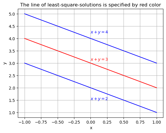
Describe all least-squares solutions of the system
𝑥+𝑦𝑥+𝑦=2=4
Solution:
Let 𝐴=[1111] , and 𝑏⃗ =[24]. We find the normal equation of 𝐴𝑥⃗ =𝑏⃗
𝐴𝑇𝐴𝑥⃗ =𝐴𝑇𝑏⃗
A = np.array([[1,1],[1,1]])

b = np.array([[2,4]]).T

#compute A^TA

ATA = A.T @ A

print('ATA = \n', ATA,'\n')

#compute A^Tb

ATb = A.T @ b
print('ATb = \n', ATb)
ATA =
 [[2 2]
 [2 2]]

ATb =
 [[6]
 [6]]
Thus, the normal equation is
whose solution is the set of all \((x,y)\) such that \(x+y = 3\). The solutions form a line midway between \(x+y = 2\) and \(x+y = 4\).
import matplotlib.pyplot as plt

# Data for plotting

x = range(-1, 2)
y1 = [ 2 - k for k in x]
y2 = [ 3 - k for k in x]
y3 = [ 4 - k for k in x]

fig, ax = plt.subplots()

# Specify the length of each axis
#ax.set_xlim(-5,5)
#ax.set_ylim(-5,5)

#Plot x and y1 using blue color
ax.plot(x, y1, color = 'b')
ax.text(0,1.5,'$x + y = 2$', color = 'b')

#Plot x and y2 using red color
ax.plot(x, y2, color = 'r')
ax.text(0,3.1,'$x + y = 3$', color = 'r')

#Plot x and y3 using blue color
ax.plot(x, y3, color = 'b')
ax.text(0,4.2,'$x + y = 4$', color = 'b')


# Add labels and a title to the graph
ax.set(xlabel=' x', ylabel='y', title = 'The line of least-square-solutions is specified by red color')
ax.grid()

plt.show()