Show code cell source
import numpy as np
import matplotlib.pyplot as plt
7.5. Optimization and Cobbs-Douglas Production#
In this lab we will consider two optimization problems related to a Cobbs-Douglas production function \(Q=AL^aK^{1-a}\) where \(Q\) is units of production, \(L=\) units of labor, \(K=\) units of capital and \(A\) and \(\alpha\) are constants. We also use a total cost function of the form \(TC=FC+c_LL+c_KK\) where \(FC=\)fixed cost, \(c_L=\) cost per unit of labor and \(c_K=\) cost per unit of capital.
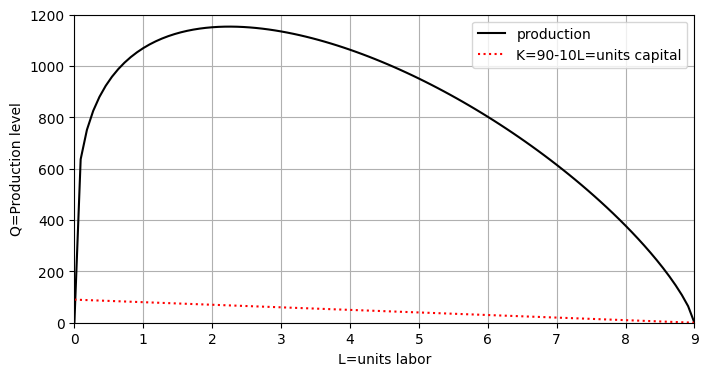
Problem 1: By constraining the total cost, we can obtain a formula for \(K\) in terms of \(L\), in which case \(Q\) becomes a function of \(L\). A plot of \(Q(L)\) shows there is a maximum value. The exact coordinates of the maximum can be obtained by setting \(\frac{dQ}{dL}\) equal to zero and solving for \(L\).
Example: Plot \(Q=40L^{1/4}K^{3/4}\) under the total cost constraint \(TC=1000 = 100 + 100L + 10K \Rightarrow K=90-10L\).
Solution: In this case, \(Q=40L^{.25}(90-10 L)^{.75}\), whose graph created in the next cell has a maximum value.
Show code cell source
L=np.linspace(0,9,100)
Q=40*(L**.25)*(90-10*L)**.75
K=90-10*L
plt.figure(figsize=(8, 4))
plt.plot(L,Q,color='k',label="production")
plt.plot(L,K,color='r',linestyle=":",label="K=90-10L=units capital")
plt.xlim((0.,9.))
plt.ylim((0,1200.))
plt.grid()
plt.xlabel("L=units labor")
plt.ylabel("Q=Production level")
plt.legend()
plt.savefig("cobbsdouglas.png")
plt.show()
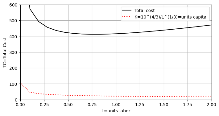
Problem 2: If we set the production level \(Q\) to be a specific value, we can solve for \(K\) in terms of \(L\) and express the total cost function as a function of \(L\) only. A plot of the total cost function \(TC(L)\) shows it has a minimum value.
Example: Plot \(TC(L,K)=100+100L+10K\) under the constraint \(Q=40L^{1/4}K^{3/4}=400 \Rightarrow K=\frac{10^{4/3}}{L^{1/3}}\).
Solution: In this case \(TC=100+100L+10^{7/3}L^{-1/3}\), and the graph created in the next cell shows there is a minimum value.
Show code cell source
L=np.linspace(.01,9,100)
K=10**(4/3)/L**(1/3)
TC=100+100*L+10**(7/3)*L**(-1/3)
plt.figure(figsize=(8, 4))
plt.plot(L,TC,color='k',label="Total cost")
plt.plot(L,K,color='r',linestyle=":",label="K=10^(4/3)/L^(1/3)=units capital")
plt.xlim((0.,2.))
plt.ylim((0,600.))
plt.grid()
plt.xlabel("L=units labor")
plt.ylabel("TC=Total Cost")
plt.legend()
plt.savefig("cobbsdouglas2.png")
plt.show()
7.5.1. Exercises#
Exercises
(Maximize Production given Total Cost) Consider the Cobb-Douglas production function \(Q=2 L^{.4} K^{.6}\). Suppose the labor input cost is \(c_L=\$10\) per unit and the capital input cost is \(c_K =\$20\) per unit. Suppose further that there is a \(\$20\) fixed cost and the firm decides it will limit the total cost to \(\$3,040\). Find the maximum production.
(Minimizing Total Cost given the Production Level) Consider the Cobb-Douglas production function \(Q=2 L^{.4} K^{.6}\) and the same cost function in problem 1. Minimize the total cost if 130 units are produced.