import pandas as pd
import numpy as np
import matplotlib.pyplot as plt
from PIL import Image
import folium # map rendering library
from folium.features import DivIcon #used to add popup info to a map
import shapely
from shapely.geometry import Point, Polygon
import shapefile # install pyshp first if you get a ModuleNotFoundError
import sklearn
from sklearn.cluster import KMeans
4.10. JNB Lab: Housing Equity Initiative#
4.10.1. Introduction#
In Fall 2021, the Housing Equity Initiative (HEI) was launched by Sunshine Gospel Ministries in partnership with The BLOCK Movement, both non-profit organizations deeply rooted in the South Side of Chicago. Housing inequity between White and Black people living in the United States is a nationwide problem. In 2020 the National Association of Realtors indicated over 70% of Whites live in their own homes, while for Blacks it is less than 45%. Based on Federal Reserve data for 2019, the real estate wealth per capita for Whites is over 140,000, but for Blacks, it is under $60,000.
In the aftermath of the Great Migration of those escaping the Jim Crow South, which brought a large influx of Blacks into Chicago in the first half of the 20th century, decades of housing-related injustices including redlining, blockbusting, restrictive covenants, and slum land-lording have occurred on the South and West sides [Amdat 2021]. Many communities affected by structural racism are carrying the burden of inequitable housing. For example, for the Woodlawn community area with roughly 9,000 housing units, almost 80% are renter-occupied, 36% of which in 2014 were using more than 50% of their income on rent. (For Woodlawn, the 2014 area median income (AMI) was roughly $25,000.)
HEI is focused on affordable home ownership in the Woodlawn area, the active construction site of the $500+ million dollar Obama Presidential Center. HEI seeks to overcome a long history of structural barriers to home ownership by providing three forms of support for vulnerable families:
Tax-Sale Benevolence Program (TSBP) to help existing homeowners avoid foreclosure due to tax sales;
Downpayment Assistance Program (DAP) to assist responsible families with down payment on a home purchase; and
Affordable Revitalization Program (ARP) to revitalize empty lots and rehab properties with well-constructed, owner-occupied homes.
HEI’s goal is not simply to increase home ownership for neighborhood residents who have experienced housing inequity, but to maximize positive, rather than negative, home ownership experiences
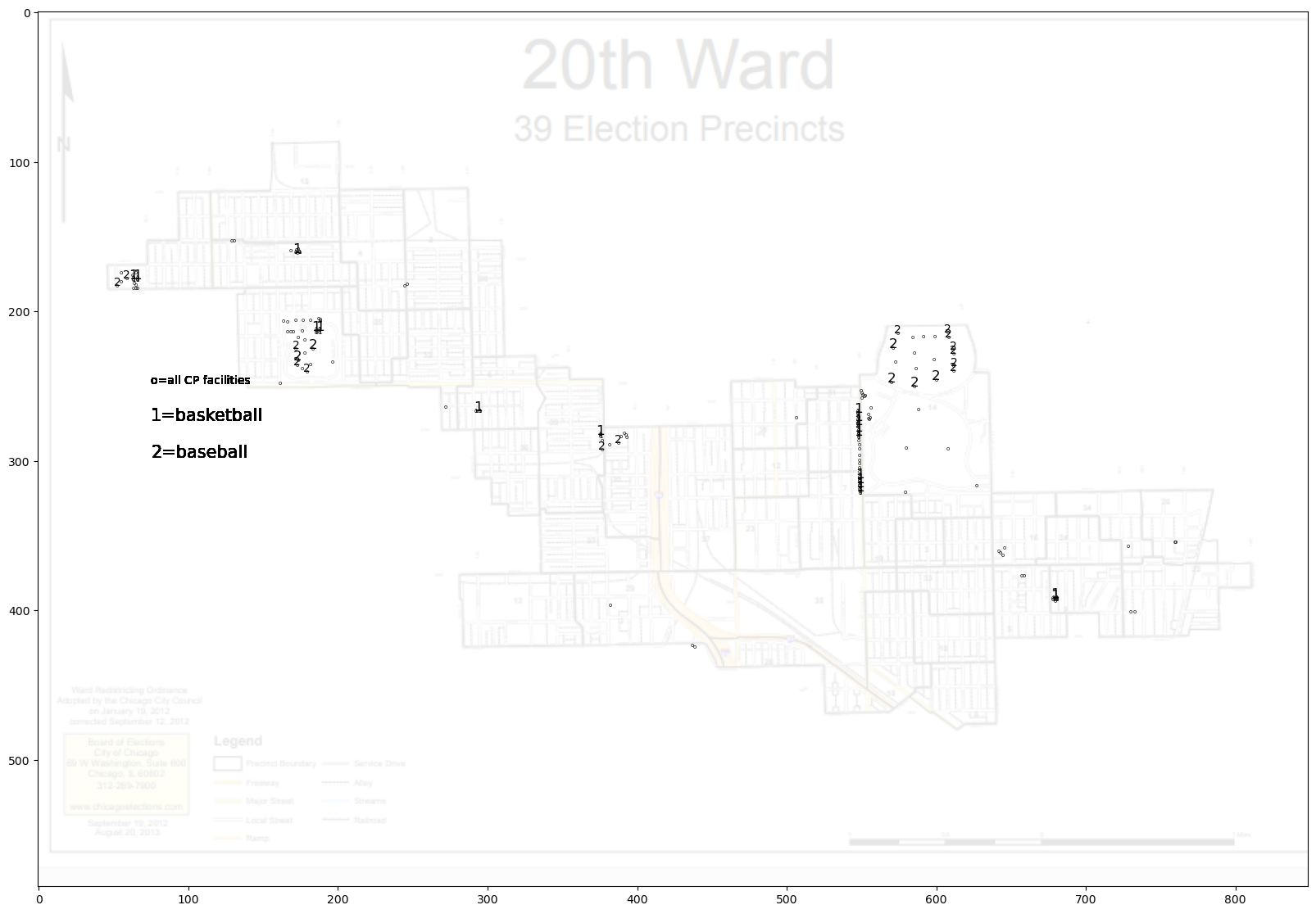
4.10.2. Park district facilities in Ward 20#
There are several factors which can make a difference in whether a young person growing up in a disadvantaged urban community will flourish. One type of community asset are park district facilities. Here we will create a map of such resources for HEI’s neighborhood.
Import Ward 20 map.
img = Image.open("ward20.png")
Define a function to convert (lat,lon) to an (x,y) location on the Ward 20 map.
#Function to convert (lat,lon) to (x,y) location on the Ward 20 map
def coord(lat,lon):
    minlon=-87.672079
    maxlon=-87.586493
    xmin=47
    xmax=806
    x=xmin+(lon-minlon)*(xmax-xmin)/(maxlon-minlon)
    minlat=41.778798
    maxlat=41.801243
    ymax=189
    ymin=389
    y=ymin+(lat-minlat)*(ymax-ymin)/(maxlat-minlat)
    return x,y
Import a shape file with the Ward 20 boundary.
sf = shapefile.Reader("ward20.shp")
shapes=sf.shapes()
Read in the Chicago Park District data from the Chicago Data Portal.
parks=pd.read_json("https://data.cityofchicago.org/resource/eix4-gf83.json?$limit=400000")
parks.head(1)
| the_geom | objectid_1 | park | park_no | facility_n | facility_t | x_coord | y_coord | gisobjid | |
|---|---|---|---|---|---|---|---|---|---|
| 0 | {'type': 'Point', 'coordinates': [-87.63769762... | 1 | HAMILTON (ALEXANDER) | 9 | CULTURAL CENTER | SPECIAL | -87.637698 | 41.762999 | 2494 |
p=parks[["facility_n","facility_t","x_coord","y_coord"]]
p.columns=["type","loc","longitude","latitude"]
p.head(3)
| type | loc | longitude | latitude | |
|---|---|---|---|---|
| 0 | CULTURAL CENTER | SPECIAL | -87.637698 | 41.762999 |
| 1 | GYMNASIUM | INDOOR | -87.637929 | 41.762817 |
| 2 | BASEBALL JR/SOFTBALL | OUTDOOR | -87.636914 | 41.760849 |
p["type"].value_counts()
type
BASKETBALL BACKBOARD         771
BASEBALL JR/SOFTBALL         537
PLAYGROUND                   517
TENNIS COURT                 507
BASKETBALL COURT             323
                            ...
GOLF COURSE MINIATURE          1
SPORT ROLLER COIRT             1
NATURE PLAY AREA               1
ALFRED CALDWELL LILY POND      1
ART TURF - REGULATION          1
Name: count, Length: 75, dtype: int64
Map the Park District data.
import matplotlib.pyplot as plt
from PIL import Image
img = Image.open("ward20.png")
plt.figure(figsize=(20,16))
plt.imshow(img,alpha=.1)
df=p

#use this format
for i in df.index:
    [x,y]=coord(df.loc[i,"latitude"],df.loc[i,"longitude"])
    point=Point(df.loc[i,"longitude"],df.loc[i,"latitude"])
    if point.within(Polygon(shapes[3].points)):
        plt.text(x,y,"o",color='black',size=5,ha='center',va='bottom')
        plt.text(75,250,"o=all CP facilities",color='black',size=10,ha='left',va='bottom')
        if df.loc[i,"type"]=="BASKETBALL BACKBOARD":
            plt.text(x,y,"1",color='black',size=5,ha='center',va='bottom')
            plt.text(75,275,"1=basketball",color='black',size=15,ha='left',va='bottom')
        if df.loc[i,"type"]=="BASKETBALL COURT":
            plt.text(x,y,"1",color='black',size=12,ha='center',va='bottom')
        if df.loc[i,"type"]=="BASEBALL JR/SOFTBALL":
            plt.text(x,y,"2",color='black',size=10,ha='center',va='bottom')
            plt.text(75,300,"2=baseball",color='black',size=15,ha='left',va='bottom')
        if df.loc[i,"type"]=="BASEBALL SR":
            plt.text(x,y,"2",color='black',size=12,ha='center',va='bottom')
plt.savefig("recreation.png")
plt.show()
Problem 1
Add playgrounds to the map in red.
4.10.3. Tax Year 2019 Owner-Occupied Tax Sale Data for Ward 20#
Import tax-sale data.
df=pd.read_excel("Ward20residentialparcels.xlsx")
df2=pd.read_excel("HEIcandidateparcels.xlsx")
Create map of Ward 20 residential parcels and HEI candidate parcels.
Chicago_map = folium.Map(location=[41.78453, -87.62859],   zoom_start=13,alpha=.1)
for i in np.arange(0,169,1):
    p=[df.loc[i,"latitude"],df.loc[i,"longitude"]]
    folium.Marker(p,icon=DivIcon(
        icon_size=(100,0),
        icon_anchor=(0,8),
        html='<div style="font-size: 2pt; color : lightgray">'+'</div>',
            )).add_to(Chicago_map)
    Chicago_map.add_child(folium.CircleMarker(p, radius=1,color='lightgray'))
for i in np.arange(0,92,1):
    p2=[df2.loc[i,"latitude"],df2.loc[i,"longitude"]]
    folium.Marker(p2,icon=DivIcon(
        icon_size=(100,0),
        icon_anchor=(0,8),
        html='<div style="font-size: 6pt; color : black">'+'   '+str(df2.loc[i,"Total Tax Due"])+ '</div>',
            )).add_to(Chicago_map)
    Chicago_map.add_child(folium.CircleMarker(p2, radius=1,color='black'))
Chicago_map.save("HEItaxsaleyear19maprev.html")
Chicago_map
Exercise
Make a histogram showing tax sale amounts for Ward 20 residential parcels and HEI candidate parcels.
4.10.4. Low Income Tract Clustering#
Read in census tract data.
rawdf=pd.read_csv("tract_covariates.csv")
rawdf.columns
Index(['tract', 'county', 'state', 'hhinc_mean2000', 'mean_commutetime2000',
       'frac_coll_plus2010', 'frac_coll_plus2000', 'foreign_share2010',
       'med_hhinc2016', 'med_hhinc1990', 'popdensity2000', 'poor_share2010',
       'poor_share2000', 'poor_share1990', 'share_black2010', 'share_hisp2010',
       'share_asian2010', 'share_black2000', 'share_white2000',
       'share_hisp2000', 'share_asian2000', 'gsmn_math_g3_2013',
       'rent_twobed2015', 'singleparent_share2010', 'singleparent_share1990',
       'singleparent_share2000', 'traveltime15_2010', 'emp2000',
       'mail_return_rate2010', 'ln_wage_growth_hs_grad', 'jobs_total_5mi_2015',
       'jobs_highpay_5mi_2015', 'nonwhite_share2010', 'popdensity2010', 'cz',
       'czname', 'ann_avg_job_growth_2004_2013', 'job_density_2013'],
      dtype='object')
rawdf.shape
(74123, 38)
Filter data to Cook County tracts with median 2016 household income <30,000.
IL=rawdf[rawdf['state']== 17]
IL.shape
(3128, 38)
cook=IL[IL['county']==31]
cook.shape
(1319, 38)
low_inc=cook[cook['med_hhinc2016']<30000]
low_inc.shape
(202, 38)
Prepare columns used for separation.
df=low_inc[['tract','emp2000', 'frac_coll_plus2010','job_density_2013',   'mean_commutetime2000', 'med_hhinc2016','popdensity2010', 'rent_twobed2015','singleparent_share2010']]
df.columns
Index(['tract', 'emp2000', 'frac_coll_plus2010', 'job_density_2013',
       'mean_commutetime2000', 'med_hhinc2016', 'popdensity2010',
       'rent_twobed2015', 'singleparent_share2010'],
      dtype='object')
df.columns=['Tract','emp','college','jobdensity','commute','hhincome','popdensity','rent','singleparent']
df.head(1)
| Tract | emp | college | jobdensity | commute | hhincome | popdensity | rent | singleparent | |
|---|---|---|---|---|---|---|---|---|---|
| 21107 | 10100 | 0.560484 | 0.349921 | 2530.6123 | 41.525024 | 29861.0 | 33020.406 | 1153.0 | 0.543056 |
df.loc[:, 'work'] = df.loc[:, 'jobdensity'] / df.loc[:, 'popdensity']
df.loc[:, 'room'] = df.loc[:, 'rent'] / df.loc[:, 'hhincome']
Normalize values
df.shape
(202, 11)
df=df.dropna()
df.shape
(167, 11)
Mwork=df["work"].max()
mwork=df["work"].min()
Mroom=df["room"].max()
mroom=df["room"].min()
Msingleparent=df["singleparent"].max()
msingleparent=df["singleparent"].min()
Mcommute=df["commute"].max()
mcommute=df["commute"].min()
Mcollege=df["college"].max()
mcollege=df["college"].min()
Mhhincome=df["hhincome"].max()
mhhincome=df["hhincome"].min()
#normalize values
df.loc[:,"work"]=(df.loc[:,"work"]-mwork)/(Mwork-mwork)
df.loc[:,"room"]=(df.loc[:,"room"]-mroom)/(Mroom-mroom)
df.loc[:,"singleparent"]=(df.loc[:,"singleparent"]-msingleparent)/(Msingleparent-msingleparent)
df.loc[:,"commute"]=(df.loc[:,"commute"]-mcommute)/(Mcommute-mcommute)
df.loc[:,"education"]=(df.loc[:,"college"]-mcollege)/(Mcollege-mcollege)
df.loc[:,"income"]=(df.loc[:,"hhincome"]-mhhincome)/(Mhhincome-mhhincome)
tracts=df[["Tract","work","room","education","income","singleparent","commute"]]
tracts.shape
(167, 7)
tracts=tracts.dropna()
tracts.shape
(167, 7)
Use k-means to separate the census tracts into two clusters.
cols=["work","room","education","income","singleparent","commute"]
tractcluster=tracts[cols]
# Fit the k means model
k_means = KMeans(init="k-means++", n_clusters=2, n_init=2)
k_means.fit(tractcluster)
#Get Labels
k_means_labels = k_means.labels_
k_means_labels
array([1, 1, 1, 1, 1, 1, 1, 1, 1, 1, 1, 0, 1, 1, 1, 1, 0, 0, 0, 0, 0, 0,
       0, 0, 0, 0, 0, 0, 0, 0, 1, 0, 0, 0, 0, 0, 1, 1, 1, 1, 1, 1, 1, 0,
       0, 0, 0, 0, 0, 1, 0, 1, 0, 1, 1, 0, 1, 0, 0, 0, 0, 0, 0, 1, 0, 0,
       0, 1, 0, 0, 0, 0, 0, 0, 1, 0, 1, 1, 1, 0, 0, 0, 0, 0, 1, 0, 0, 1,
       0, 1, 1, 1, 1, 1, 0, 1, 0, 1, 0, 0, 0, 0, 0, 0, 1, 1, 0, 0, 0, 0,
       0, 0, 0, 0, 0, 0, 1, 0, 0, 0, 1, 0, 0, 0, 1, 1, 1, 0, 0, 1, 1, 1,
       0, 1, 0, 1, 1, 1, 1, 0, 1, 0, 1, 0, 0, 0, 1, 0, 0, 1, 1, 1, 0, 0,
       1, 1, 1, 0, 0, 0, 1, 0, 0, 0, 1, 1, 1], dtype=int32)
tracts["CLASS"]=k_means_labels
tracts=tracts.reset_index(drop=True)
tracts.head(2)
| Tract | work | room | education | income | singleparent | commute | CLASS | |
|---|---|---|---|---|---|---|---|---|
| 0 | 10100 | 0.012277 | 0.228804 | 0.423649 | 0.994194 | 0.491649 | 0.554853 | 1 |
| 1 | 10202 | 0.043318 | 0.222477 | 0.280312 | 0.973262 | 0.617686 | 0.401514 | 1 |
C0=tracts[tracts["CLASS"]==0]
C0.head(1)
| Tract | work | room | education | income | singleparent | commute | CLASS | |
|---|---|---|---|---|---|---|---|---|
| 11 | 231200 | 0.012669 | 0.1637 | 0.129681 | 0.843523 | 0.733 | 0.707592 | 0 |
C1=tracts[tracts["CLASS"]==1]
C1.head(1)
| Tract | work | room | education | income | singleparent | commute | CLASS | |
|---|---|---|---|---|---|---|---|---|
| 0 | 10100 | 0.012277 | 0.228804 | 0.423649 | 0.994194 | 0.491649 | 0.554853 | 1 |
C0.shape
(96, 8)
C1.shape
(71, 8)
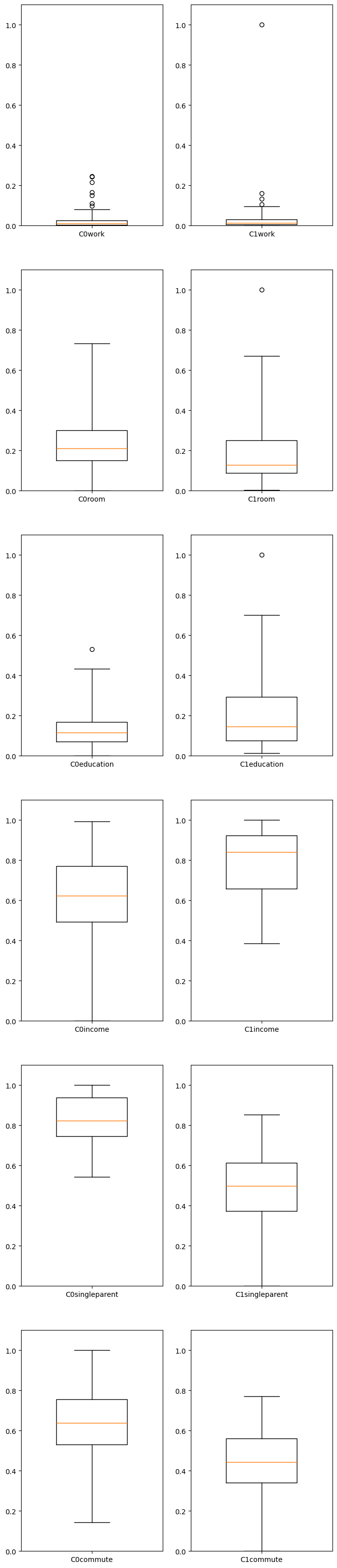
Make a boxplot comparison of the two groups
numplots=len(cols)
plt.figure(figsize=[10,numplots])
fig, axes = plt.subplots(numplots,2,figsize=[8,40])
for i in np.arange(0,numplots,1):
    axes[i,0].set_ylim((0,1.1))
    axes[i,1].set_ylim((0,1.1))
    axes[i,0].boxplot(C0[cols[i]],whis=3,labels=['C0'+cols[i]],widths=.5)
    axes[i,1].boxplot(C1[cols[i]],whis=3,labels=['C1'+cols[i]],widths=.5)
fig.savefig('6IndR1.png') #Save our figure to a file
plt.show()
<Figure size 1000x600 with 0 Axes>
df2.shape
(92, 34)
Exercise
Continue the same process one further step starting with the sub-cluster (C0 or C1) that exhibits greater hardship.