3.3. Working with Data#
3.3.1. Introduction#
In this section, we will bring the Python programming part to be more related to data processing. The organization of this section is as follows: First, we will begin with an overview of data, describe the background of processing data, and explore various data types. Then, we will show how the Python programming language is written to prepare the data for analysis, including reading and writing data. Next, we will specifically introduce pandas, a data analysis library in Python, to demonstrate the ways of data processing and data operations for statistics and analysis. Finally, we will guide you through the basics of Matplotlib, a popular Python library for data visualization.
3.3.2. An Overview of Data and Data Analysis#
There are several data-related research areas. A database researcher is interested in how data is stored and managed, whereas a data scientist focuses more on the topics such as methods of processing massive data, analyzing data from various sources, interpreting analyzed data, and visualizing the analytical results. Data analysis, in particular, has drawn attention to statisticians, computer scientists, business people, health professionals, or even philosophers and artists.
Traditionally, data analysis was thought to be done by mathematicians only. Scholars often considered it in the domain of statistics. Today, however, new challenges motivate us to think of data analysis as a broad, multidisciplinary area. We use a variety of tools including computer programs to perform data operations. Due to the scope of this chapter and this book, we describe only a few facts of data and its related challenges in the era of modern data analysis.
At present, scholars are dealing with large-scale data everywhere. For example, the Internet today has billions of webpages. According to the conservative estimates, there are at least three hundred billion emails that are sent daily. The need of analyzing such a great amount of data effectively has driven scientists to develop well-designed methods and to constantly update the hardware to increase the computing power.
The modern world generates data at a fast pace. Even if the data is from the same source, numbers that are collected in the past can be very different from them at present. At the early stage of the COVID-19 pandemic, researchers and decision makers realized that the reported data of disease infections fell behind. The collected data for the daily reporting largely reflected what had happened in the past rather than what was happening.
Data analysts are presented with structured, semi-structured, or unstructured data. One example of a structured dataset may be from a professor’s grade book. Students’ names and grades of all assignments are presented completely and accurately in a well-organized and cross-checked spreadsheet/table. Less or no additional effort of data “re-structuring” needs to be made. However, data from an ordinary person’s diary can be unstructured. The personal note has various lengths, covers different and unrelated topics, and is likely handwritten. Extracting data for an analytical process requires a tremendous amount of data pre-processing work.
Just like water is an important resource for people, agriculture, and industry, data is everywhere and fundamental in many different contexts. However, just like water, the origin and the quality of data matter. The prevalence of data does not imply that all kinds of data can be used without scrutiny. An online survey result that was collected anonymously and assembled by a controversial business entity may be a less reliable and more biased source for data analytics. The clinical trial data submitted by responsible medical professionals and peer reviewed by a reputable research group is thought to be more trustworthy for academic purposes. The extent of data pre-processing depends on the source and the collection method of data.
There are various features of data due to the difference of dataset size, generation method, structure, and its sources. For analyzing data, several methods and challenges exist, too. The direction of data analysis can be predictive or descriptive:
For predictive data analysis, one uses existing data to predict unknown and future data. For example, a credit card company can analyze the history of a user’s credit card use to detect potential fraud and possibly unauthorized transactions. An economist may analyze data from multiple sources to model the likelihood of a recession in the next few weeks or months. A climate scientist is able to create a model to predict the temperature trend from a region based on the historical pattern of the climate data.
For descriptive data analysis, one performs analysis on available data in order to discover and better understand the features of the dataset. For example, a genealogist may use a program to analyze the people’s faces to tell how two individuals look similar to or different from each other. A business sales team may perform a market basket analysis from millions of transactions to discover the sets of frequently brought items.
The choice of a data analysis method depends on not only the objective of analysis but also the type of data.
Generally speaking, there are four common types of data [S.S.Stevens].
Nominal data is the names or values themselves, such as postal codes or identification numbers.
Ordinal data affords a natural ordering or ranking, such as wine’s quality grades or customer’s satisfaction ratings.
Interval data also can be ordered, but in this case the difference of data values is more explainable—calendar dates, for example.
Ratio data can be meaningfully multiplied or divided, such as the distance between two locations.
Data operations must be suitable for the specific data types. We can say that iron is about 7.8 times as heavy as water (the density of iron is 7.87 g/\(m^{3}\); the density of water is 1 g/\(m^{3}\)). However, it is wrong to do a simple arithmetic sum operation by saying the density of a mixture of iron and water is 8.8 (as 7.8+1) times as heavy as water. In biology, a DNA molecule is composed of four types of bases: adenine (A), thymine (T), guanine (G), and cytosine (C). These four bases are paired as A to T and G to C. However, we cannot just “compare” them to determine which base is “larger” or “precedent” of another, in the usual way that we do with natural numbers.
In the next part of this chapter, we will cover data analysis topics from executing common statistical tasks to building specific models for further analysis. We will demonstrate to the readers how to write Python programs relevant to the theoretical aspect of analysis. Moreover, we will discuss the benefits of utilizing computer programs when the data is processed with the help of Python libraries.
*: Stevens, S. S. (1946). On the theory of scales of measurement. Science, 103(2684), 677-680.
3.3.3. Data Operations: Importing and Exporting, Reading and Writing Data#
For the complete process of data analysis, programmers usually follow the sequence of:
Reading data from a file or from the user input,
Processing loaded data, including re-organizing data, computations, and generating results,
Outputting data to the computer screen or writing the output to files.
The first step is pre-processing the data, that is, to prepare the “clean” data for analysis from the raw data. This step usually involves the loading of a dataset that is imported from databases, files, or the user inputs. The raw data can take various forms. As we have mentioned in the previous section, the data can be more or less structured. In this chapter, we will focus on the processing of structured datasets.
A structured dataset, according to this book’s definition and its applications, is the one that is:
Linear, such as a collection of records with the same type, i.e. 1-dimensional data, or
Table-like, such as the records organized with complete information of rows and columns, i.e. 2-dimensional data, or
Cuboid-like, such as data points in a space, represented by three values, x, y, z, i.e. 3-dimensional data).
Since the computer screen is “flat”, i.e. 2-dimensional, and all data must be properly structured and saved into the memory space, we still need to convert the 3-dimensional data in a form that fits into a 2-dimensional data’s view. There are several techniques that do such kind of 3D-to-2D conversion, but this topic is currently beyond the scope of our book. Therefore, we only introduce the methods of processing a file that is already saved with one dimension or two dimensions.
One-dimensional data processing#
For a one-dimensional dataset, a Python program can read the data from the user input one at a time. The program may save all user-inputted data into a data structure such as a list.
###########------uncomment this block if working with an interactive JNB-------------###############

## The program asks the number of inputs by the user
# print("How many numbers to input")

# num_inputs = int(input()) # The input() function takes a string by default. Converting to int type.
# data_list = []   # Initial list is empty

## The user inputs records one after one. All will be saved into data_list
# print("Enter each record. Press Enter to continue.")
# for i in range(num_inputs):
#    user_data = input()
#    data_list.append(user_data)

##########---------------------------------------------------------------------------################

#delete the following line if running an interactive JNB
data_list=[4,6,8,2,21,9,5]


# Output the list that contains all previously inputted data
print(data_list)
[4, 6, 8, 2, 21, 9, 5]
Another situation to read the data is from a file. For the convenience of processing, we assume that such a file is a plain text file and it only contains relevant data for calculations (i.e. no data labels, titles, informational fields, or any empty spaces or lines). Furthermore, we assume that all records are stored in one line where the two records are separated by a single white space.
# First, open the file that contains all records; store the content to the object data_file_1.
data_file_1 = open("datafile1.txt", "r")

# Then, read the data_file object for the first (also the only and the last) line and save it to a string.
one_line = data_file_1.readline()

# Next, split the string into several records and further save the records into a list.
# Note: the white space is the separator in this program.
data_list = one_line.split()

# Finally, output the data from the saved list, data_list.
print(data_list)

# Close the file.
data_file_1.close()
['7', '12', '41', '3', '19', '24', '81']
Explanation:
The file open() function in this code example takes two arguments. The first one is the file name. The second one is the file processing mode. “r” here means read. The readline() function outputs only one line of data from a file if it is used once.
The split() function is used to split data based on the separator. If nothing is specified in the function’s argument, the default separator is white spaces.
As a good programming practice, programmers should close the file before the end of the program by explicitly writing the file closing function close().
On the other hand, we can assume that the data are stored in multiple lines where each line contains one record.
# First, open the file that contains all records; store the content to the object data_file_2.
data_file_2 = open("datafile2.txt", "r")

# Next, use a loop to iterate all lines, where each line has one record.
for line in data_file_2.readlines():
    # Output data
    print(line[:-1]) # -1 is used for not printing the end-of-line’s line break character

# Close the file.
data_file_2.close()
7
12
41
3
19
24
81
Explanation:
The readlines() function differs from the readline() function. The program will continue to read another line till the end of the file. The for loop is used to iterate each line. The print() function inside the for loop will print each line’s content except the line break character at the end of each line.
This program treats each line as a string. The code line[:-1] means that the program does slicing of the string so that the new string contains all characters from the beginning to the second-to-last character, cutting off the last. The value -1 used as an index means the last position, and :-1 indicates that the last position is an exclusive upper bound.
When reading a plain-text file, the last character on a line is the line break itself, and so line[:-1] simply gets rid of the line break character.
In most programming languages, including Python, such a line break character is represented by \n. That \n is not a part of data itself and thus should be removed. Please note that we must ensure that the last record or line of the file is also followed by a line break (\n) or that record will not be processed correctly.
Two-dimensional data processing#
An efficient way of storing the data in a table (i.e. two-dimensional data) is using a file format called Comma-Separated Values (CSV). Such a file is named like birds.csv. A typical .csv file looks like the following:
# Import the pandas library. Here we rename "pandas" as "pd" for convenience.
import pandas as pd

# Read and load the .csv data from the specified file location into the program's memory space,
# and save the data into a format called "DataFrame".
my_data = pd.read_csv('birds.csv')

# Operate on the object with the DataFrame format.
print(my_data)
                      Name  Weight  Clutch size  Wingspan     Family (common)  \
0       American goldfinch    15.5            5      20.5             finches
1           American robin    83.0            4      36.5            thrushes
2   black-capped chickadee    11.5            7      18.5                tits
3                 blue jay    85.0            4      38.5             corvids
4         eastern bluebird    30.0            4      28.5            thrushes
5            mourning dove   141.0            2      41.5   doves and pigeons
6        northern cardinal    45.0            4      28.5           cardinals
7        redwing blackbird    54.5            4      14.5          blackbirds
8         Baltimore oriole    35.0            4      27.5          blackbirds
9          dark-eyed junco    24.0            4      21.5  new-world sparrows
10         common starling    78.0            6      37.5           starlings

   Family (scientific)
0         Fringillidae
1             Turdidae
2              Paridae
3             Corvidae
4             Turdidae
5           Columbidae
6         Cardinalidae
7            Icteridae
8            Icteridae
9        Passerellidae
10           Sturnidae
Explanation:
On line 1, we import the Pandas library, but we may not want to write the complete name of pandas every time when we use it. Therefore, we use the alias pd to denote pandas.
On line 2, my_data is the object with the DataFrame format. It is used to be processed by the Pandas library according to the row and column information. pd.read_csv is the function from the Pandas library to read the .csv file. Enclosed in the function’s parameter ‘data.csv’ is the file name (data.csv).
If your Python’s workspace and the data file are in the same directory/folder, no further action is needed from this part. However, if the data file is stored elsewhere, we must specify the location of such a file in the Python code, such as:
my_data2 = pd.read_csv('user/math_teacher/Desktop/project2/data2.csv')
or
my_data3 = pd.read_csv('C:\\Users\\Math_Student\\Desktop\\Project3\\data3.csv')
Note that the Python code for specifying a file location depends on the operating system the user is using. The first form is usually suitable for MacOS and Linux systems, where a forward slash (/) is used to go into a sub-directory. The second form is often seen in a system where a backward slash (\) is used to go into a sub-directory, such as Microsoft Windows. Here, two backward slashes are used because Python processes the special character \ with an escape character . The first \ is for the formatting purpose to indicate that there is a special character coming next and the second \ is the actual character to be read.
As the file name has suggested, the file contains comma-separated values because commas (,) are commonly used to separate the columns. However, files can still be processed by the Python program if the columns are separated by a symbol other than a comma. Such a symbol may be a white space ( ), a semi-colon (;), or any other symbol.
In order to read such kind of file and process the column information correctly, we change the parameter part “sep=X” to indicate a different separator. “X” is replaced by the separator.
For example,
my_data4 = pd.read_csv('data4.csv', sep = ' ')
or
my_data5 = pd.read_csv('data5.csv', sep = ';')
From the above examples, the first one is used to process a file where columns are separated by a single white space. The second one is by a semi-colon. If no parameter is specified, this read_csv function will process the file that treats the comma as the separator by default.
Exporting Data: Writing Data to A File#
Next, we describe the ways to export and present data. If the output is to the computer screen, Python’s print() function should have the need. If we want to output data to a file, we will use Python’s file writing functions. The following code can be used to write the data to a file. At this time, we also assume that the file is in a plain text format, which is more conventional and convenient for the data storage, other than a binary format, which is encoded for the use by a computer program and/or program instructions.
# Assuming that all generated data have been stored in a list….
generated_data = [10, 20, 30, 4, 5, 6]

# First, open the file to which the data is being written to
output_file = open("results.txt", "w")

# Next, iterate all elements in the list so that each element is written to the same file
for i in generated_data:
    output_file.write(str(i) + " ") # elements one after one, separated by a white space.

# Close the file.
output_file.close()
Explanation:
In this example, we assume that all data have already been stored in a list. Since the file operation is to write to a file, we use the parameter “w” within the open() function to write data to a file. results.txt is the plain text file name that all data is written to.
The program will process the for loop by accessing each element in the list one by one. In each iteration of the loop, the program executes the write() function by pushing one element into the file. The file writing function, write(), always needs to process strings only (the system treats the output as a long string) but the user generated data may not be strings. Just like in our example, we must convert the number type data, e.g. int, into a string type. Therefore, we use str() to do such a type conversion.
After one element is written into the file, a white space is also written to the file before the loop repeats to write another element into the file. Finally, the program closes the file with the close() function.
The code example works to output all data into a file, where all records are stored in one line only. What if the user intends to output data with multiple lines, where each line contains one record only? What if the user decides to save the output file in a directory other than the Python program’s default working directory? We are leaving these questions to the readers.
3.3.4. Introduction to Pandas#
The code in the previous section used the pandas library to read csv data. But pandas does a lot more, and in fact is one of researchers’ top selections of libraries for its
convenience and effectiveness in performing data analysis. According to the official website, pandas “is a fast, powerful, flexible and easy to use open source data analysis and manipulation tool, built on top of the Python programming language.”(https://pandas.pydata.org/) The letters from the library’s name appear to be taken from “Python Data ANAlySis” by its creator.
pandas can be used to process datasets with various dimensions and structures. They include a one-dimensional dataset – processed as Series, a two-dimensional dataset – processed as Dataframe, a traditionally more structured dataset such as a .csv file, or a more complex but less structured dataset, such as a .json file. Users who are familiar with other programming languages and statistical applications, including R, SAS, Stata, SQL, and spreadsheets will find similar tools and operations of processing data in pandas.
Users in pandas can structure the data to be compatible with a spreadsheet software application (e.g. Microsoft Excel, LibreOffice Calc, Apple Numbers). Here are the important pandas data structures and their equivalent names in a spreadsheet application:
Series – column
Dataframe – entire worksheet
Index – row headings
NaN – empty cell
As we see, Panda’s Series is used to store and process a list of elements, i.e. data from one column. Dataframe is suitable to process data from a table. In the next section, we will explain the data operations associated with pandas Series and Dataframe.
Data operations with pandas.Series#
The Pandas library has its built-in functions to process one-dimensional data and two-dimensional data. To perform a variety of tasks with a one-dimensional dataset, we use the functions from pandas.Series. The following example shows how we load a list of elements into the Series.
import pandas as pd
# Original data are stored in a list.
data_list = [100, 200, 300, 123, 654, 99, 98, 100, 45, 100, 101]
# New data to be stored in a Series, namely data_series
data_series = pd.Series(data_list)
# Print elements from Series.
print(data_series)
0     100
1     200
2     300
3     123
4     654
5      99
6      98
7     100
8      45
9     100
10    101
dtype: int64
Notice the output from the print() function. Values from the first column are viewed as the Series index numbers, which start from 0. The second column contains the actual records from the Series data. Because the list is a one-dimensional dataset, the index value has no additional meaning other than telling the user the position (by zero-based indexing) of an element. While it is certainly possible to operate on data using Python’s list structure, including writing codes and calculating numbers, Panda’s Series has an advantage as it has provided many commonly used functions for mathematical purposes.
Following the previously made code, we can use available tools from pandas.Series to quickly get useful statistical results.
# Getting the maximum value from the series
data_series.max()
654
# Getting the minimum value from the series
data_series.min()
45
# Getting the mean value from the series
data_series.mean()
174.54545454545453
# Getting the median value from the series
data_series.median()
100.0
# Getting the mode(s) of the Series.
# A series may have multiple modes, i.e. more than one value appears the most often.
data_series.mode()
0    100
dtype: int64
# Getting the nth largest values from the series, using .largest(n).
n = 5
data_series.nlargest(n)
4     654
2     300
1     200
3     123
10    101
dtype: int64
# Getting the nth smallest values from the series, using .smallest(n).
n = 4
data_series.nsmallest(n)
8     45
6     98
5     99
0    100
dtype: int64
# Getting the standard deviation from the series.
# Such a standard deviation is normalized by N-1 by default.
data_series.std()
173.0169723676632
# Getting the variance from the series
data_series.var()
29934.87272727273
# Getting a quick statistical summary of data from the series
data_series.describe()
count     11.000000
mean     174.545455
std      173.016972
min       45.000000
25%       99.500000
50%      100.000000
75%      161.500000
max      654.000000
dtype: float64
# Getting the unique elements from the series
data_series.unique()
array([100, 200, 300, 123, 654, 99, 98, 45, 101])
# Getting the number count of unique elements from the series
data_series.nunique()
9
# Getting the size of its series, i.e. how many elements in this series
data_series.size
11
Note that when programmers write the code to get the series’ size, they write .size instead of .size(). This is because size is a data attribute (or instance variable) of
the Seires class. Recall from the introduction to classes and objects in the previous chapter that classes have both data attributes and function attributes (or methods).
Attributes such as max() and min() are defined as methods because they are actions that are performed on data. An action has its internal processing procedure and may have an output following its processing. For example, max() has its internal processing procedure that compares the values of all records and selects the maximum value. Then, it outputs the selected maximum value. Thus, we will use the output number from the max() function.
Data operations with pandas.Dataframe#
If the dataset is two-dimensional, we rely on Pandas’s Dataframe to process it. We have explained the use of Pandas library to read and extract information from a .csv file in the previous section of the chapter. Now, we will demonstrate how to use Dataframe to select and operate on the two-dimensional data.
To demonstrate the operations with panda’s Dataframe, we use the dataset from Car Evaluation Database that is downloadable from UCI Machine Learning Repository (https://archive.ics.uci.edu/dataset/19/car+evaluation). First, we download the .zip package that contains the dataset file “car.data”. Next, we change the file name from “car.data” to “car.csv”. This step is optional in the real-world data analysis since the file has already been perfectly formatted with comma-separated values. We do the file name change only for consistency in our explanation. Then we modify the file by adding a title line for our data processing need:
buying,maint,doors,persons,lug_boot,safety,class
This step can be done manually by opening the data file or by writing a line of Python code, which we will demonstrate shortly.
This dataset was originally used for predicting a car’s acceptability level based on several conditions of that car. Each row shows the conditions (attributes) and acceptability level (class value). As we look into the dataset, the Car Evaluation Database contains the following information:
Class values:
unacc, acc, good, vgood
Explanation:
class (acceptability level: unacceptable, acceptable, good, and very good).
Attributes:
buying: vhigh, high, med, low.
maint: vhigh, high, med, low.
doors: 2, 3, 4, 5more.
persons: 2, 4, more.
lug_boot: small, med, big.
safety: low, med, high.
Explanation:
buying (buying price: very high, high, medium, and low),
maintenance (price of maintenance: very high, high, medium, and low),
doors (number of doors: 2, 3, 4, and 5 or more),
persons (capacity in terms of persons to carry: 2, 4, and more),
lug_boot (the size of luggage boot: small, medium, and big), and
safety (estimated safety of the car: low, medium, and high).
# Use of Dataframe in pandas

import pandas as pd
#   Loading the dataset to let pandas read the .csv file.
loaded_data = pd.read_csv('car.csv')  # or loaded_data = pd.read_csv('car.data') for the original file name

# data_car has its title added. All column names are specified in this step.
data_car = pd.DataFrame(loaded_data, columns = ['buying','maint','doors','persons','lug_boot','safety','class'])

# Displaying the overview of the dataset
print(data_car)

# Selecting and displaying the data from the column 'buying'
print(data_car['buying'])
     buying  maint  doors persons lug_boot safety  class
0     vhigh  vhigh      2       2    small    low  unacc
1     vhigh  vhigh      2       2    small    med  unacc
2     vhigh  vhigh      2       2    small   high  unacc
3     vhigh  vhigh      2       2      med    low  unacc
4     vhigh  vhigh      2       2      med    med  unacc
...     ...    ...    ...     ...      ...    ...    ...
1723    low    low  5more    more      med    med   good
1724    low    low  5more    more      med   high  vgood
1725    low    low  5more    more      big    low  unacc
1726    low    low  5more    more      big    med   good
1727    low    low  5more    more      big   high  vgood

[1728 rows x 7 columns]
0       vhigh
1       vhigh
2       vhigh
3       vhigh
4       vhigh
        ...
1723      low
1724      low
1725      low
1726      low
1727      low
Name: buying, Length: 1728, dtype: object
One can select specific row(s) and columns from the Dataframe by using loc (to be understood as “location”) or iloc (to be understood as “index-location”) subscripts. loc is used when a label is present for rows and columns. iloc is used when the selection is based on the index values of rows and columns.
To use iloc, the subscript [ ] takes the following format: [R : C], where R is the row index and C is the column index, or [R1:R2, C1:C2], where R1 is the starting row, R2 is the ending row minus one, C1 is the starting column and C2 is the ending column minus one. If any variable, R1, R2, C1, or C2 is left blank, the selection is by default from the first row or column to the last row or column. Note that the row information and structure (the colon “:”) must be present, but the column part is optional.
Here are examples of making selections of rows and columns.
# Selecting one row, row index 5 from the dataset
data_car.iloc[5, ]
buying      vhigh
maint       vhigh
doors           2
persons         2
lug_boot      med
safety       high
class       unacc
Name: 5, dtype: object
# Selecting 3 rows from index 7 to index 9 (i.e. 10 minus 1) from the dataset
data_car.iloc[7:10, ]
| buying | maint | doors | persons | lug_boot | safety | class | |
|---|---|---|---|---|---|---|---|
| 7 | vhigh | vhigh | 2 | 2 | big | med | unacc |
| 8 | vhigh | vhigh | 2 | 2 | big | high | unacc |
| 9 | vhigh | vhigh | 2 | 4 | small | low | unacc |
# Selecting one column, column index 2 from the dataset
data_car.iloc[ : , 2]
0           2
1           2
2           2
3           2
4           2
        ...
1723    5more
1724    5more
1725    5more
1726    5more
1727    5more
Name: doors, Length: 1728, dtype: object
# Selecting 2 columns from index 2 to index 4 (i.e. 5 minus 1) from the dataset
data_car.iloc[ : , 2:5]
| doors | persons | lug_boot | |
|---|---|---|---|
| 0 | 2 | 2 | small |
| 1 | 2 | 2 | small |
| 2 | 2 | 2 | small |
| 3 | 2 | 2 | med |
| 4 | 2 | 2 | med |
| ... | ... | ... | ... |
| 1723 | 5more | more | med |
| 1724 | 5more | more | med |
| 1725 | 5more | more | big |
| 1726 | 5more | more | big |
| 1727 | 5more | more | big |
1728 rows × 3 columns
# Selecting 4 rows from index 4 to index 7 and 3 columns from index 1 to index 3 from the dataset
data_car.iloc[4:8, 1:4]
| maint | doors | persons | |
|---|---|---|---|
| 4 | vhigh | 2 | 2 |
| 5 | vhigh | 2 | 2 |
| 6 | vhigh | 2 | 2 |
| 7 | vhigh | 2 | 2 |
If one does not want to select continuous rows or columns, a Python loop may be applied to meet the selection need. Take a look at the following example.
# Iterating through each row; selecting index column 0 and 2 respectively.
for i in range(10):
  print(data_car .iloc[i, 0], data_car.iloc[i, 2])
vhigh 2
vhigh 2
vhigh 2
vhigh 2
vhigh 2
vhigh 2
vhigh 2
vhigh 2
vhigh 2
vhigh 2
# Using value_counts() to get counts of attributes
data_car['buying'].value_counts()
med      432
high     432
low      432
vhigh    432
Name: buying, dtype: int64
# Getting the unique elements from a column, e.g. 'lug_boot', using .unique()
data_car['lug_boot'].unique()
array(['small', 'med', 'big'], dtype=object)
# Getting the number count of unique elements from a column, e.g. 'lug_boot', using nunique()
data_car['lug_boot'].nunique()
3
# Getting the number count of elements for each column
data_car.count()
buying      1728
maint       1728
doors       1728
persons     1728
lug_boot    1728
safety      1728
class       1728
dtype: int64
# Getting the total number count of elements from all columns (i.e. the entire dataframe)
data_car.size
12096
3.3.5. Basics of matplotlib#
There is an old saying, a picture is worth a thousand words. Data visualization enables a reader to perceive and process information in a visualized form. Technically, data visualization transforms numerical data into a visual form. It facilitates both professionals and the general public to understand complex analytical results. Moreover, it is an important and interesting topic for data analysis.
There are several dedicated Python libraries for data visualization, including Matplotlib, Plotly, and Altair. In this section, we will talk about data visualization in general and describe the basic use of Matplotlib for plotting charts. More information about the use of Matplotlib can be found from its official website: https://matplotlib.org/
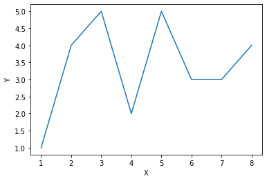
In this chapter, we will focus on the creation, description, and comparison of two-dimensional charts. Let’s take the first example of visualization with Matplotlib. The following code creates a line chart from the (x,y) pairs of data.
# Example 1: A line chart
# import matplotlib.pyplot for visualization
import matplotlib.pyplot as plt
# data for pairs x and y
x_values = [1, 2, 3, 4, 5, 6, 7, 8]
y_values = [1, 4, 5, 2, 5, 3, 3, 4]
# plotting and labeling
plt.plot(x_values, y_values)
plt.xlabel('X')
plt.ylabel('Y')
plt.show()
Explanation: matplotlib is a giant package that includes lots of visualization sub-packages and functions. We may specify the collection of functions that will be used in plotting charts, such as line charts, pie charts, etc. Therefore, we import matplotlib.pyplot instead of matplotlib so that we do not have to repeatedly write pyplot when we use its functions. Since matplotlib.pyplot is a relatively long name, we conventionally use the shorter name plt to substitute it for convenience.
The plot90 function does the visualization, and xlabel and ylabel are used for the naming of x-axis and y-axis. Finally, we use the show() function to let the chart display in the Jupyter Notebook.
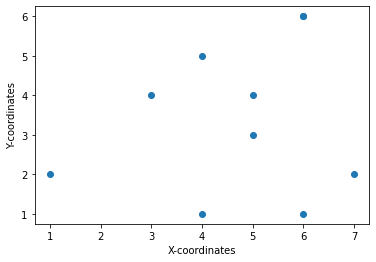
In a line chart, data points are connected by lines. We generally use a line chart when there are continuous data, e.g. stock price changes, heart rate monitoring. Occasionally, data points should not be connected as they are independent values, such as location coordinates. A scatter plot will be suitable for this kind of display.
# Example 2: a scatter plot
# import matplotlib.pyplot for visualization
import matplotlib.pyplot as plt
# Integrate matplotlib displays with Jupyter
%matplotlib inline


# data for pairs x and y
x_points = [1, 3, 4, 4, 5, 5, 6, 6, 6, 7]
y_points = [2, 4, 1, 5, 4, 3, 6, 6, 1, 2]
# plotting and labeling
plt.scatter(x_points, y_points)
plt.xlabel('X-coordinates')
plt.ylabel('Y-coordinates')
plt.show()
Sometimes, users prefer implementing charts using arrays from the Numpy library (see the previous chapter) instead of lists. We can re-write the above code to use Numpy arrays.
# Example 2.1 : a scatter plot, data from numpy
# import matplotlib.pyplot for visualization, numpy for arrays of data
import matplotlib.pyplot as plt
import numpy as np
# data for pairs x and y
x_points = np.array([1, 3, 4, 4, 5, 5, 6, 6, 6, 7])
y_points = np.array([2, 4, 1, 5, 4, 3, 6, 6, 1, 2])
# plotting and labeling
plt.scatter(x_points, y_points)
plt.xlabel('X-coordinates')
plt.ylabel('Y-coordinates')
plt.show()
Explanation: Just as we deal with matplotlib.pyplot, we conventionally take numpy as np for convenience. All data from x_points and y_points are incorporated into Numpy’s array structures. With np.array, all data points are stored and processed in a similar manner as with Python’s basic arrays.
# Example 3: plotting a sine wave
# import matplotlib.pyplot and numpy
import matplotlib.pyplot as plt
import numpy as np
# Specifying the range of x, starting value, ending value, and intervals
x_range = np.arange(-9, 9, 0.1)
# Applying the sine wave
y = np.sin(x_range)
plt.plot(x_range, y)
plt.show()
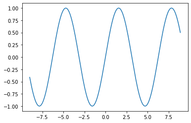
Explanation: From the above code, numpy’s arange() function takes three parameters. The first two determine the range of x values for displaying the sine wave. The third parameter is the intervals between two data points. A sine function itself treats and outputs continuous data but our Python’s code still deals with the “dots” of data with numpy. Therefore, we make the plot look like a curved data by placing a sufficient number of data points. The curve will look smooth if more points are added or rough if fewer are there. An interval of 0.1 as shown in the example means that the there is a distance of x=0.1 between two data points. x_range can be viewed as time and y can be viewed as amplitude.
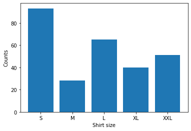
Another useful chart in visualization is the bar chart. Data from different categories may be presented with a bar chart. For example, a business would like to display the count of different shirt sizes from the its inventory. The following code does its job by a bar chart.
# Example 4: plotting a bar chart
# import matplotlib.pyplot and numpy
import matplotlib.pyplot as plt
import numpy as np
# Specifying x as catagories and y as value counts for its related catagory
x_cat = np.array(["S", "M", "L", "XL", "XXL"])
y_counts = np.array([93, 28, 65, 40, 51])
# Displaying the bar chart with labels
plt.bar(x_cat, y_counts)
plt.xlabel("Shirt size")
plt.ylabel("Counts")
plt.show()
If one needs to present data with a horizontal bar, we can simply replace the .bar() function with .barh(), as plt.barh(x_cat, y_counts).
Both the bar chart and the line chart are used to represent quantitative data. Both may be suitable to display continuous data. However, a bar chart should be chosen if such data is discrete data.
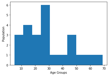
Similar to a bar chart, a histogram is used for displaying the distribution of data frequencies. Although a bar chart and a histogram look similar and both are used in statistical representation of data, there are differences. In a histogram, bars are next to each other without any interval. A histogram is a graphical representation of quantitative data, such as non-discrete data, whereas a bar chart is of categorical data.
We demonstrate a histogram with the following example. It is for displaying the population among age groups in an area.
# Example 5: plotting a histogram
# import matplotlib.pyplot and numpy
import matplotlib.pyplot as plt
import numpy as np
# Specifying ages
ages = np.array([14, 30, 20, 31, 27, 25, 21, 9, 30, 45, 25, 58, 17, 69, 16, 40, 8, 13, 44, 51, 27, 49, 19, 5])
# Displaying the histogram with labels
plt.hist(ages)
plt.xlabel("Age Groups")
plt.ylabel("Population")
plt.show()
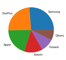
What if a user wants to present the data that will better display the ratio of each of the categories instead of the absolute value of them? A pie chart may be a good choice. Data values presented in the example are purely fictional and do not reflect any market share in any region in the real world.
# Example 6: plotting a pie chart
# import matplotlib.pyplot and numpy
import matplotlib.pyplot as plt
import numpy as np
# Specifying shares of the brands and the names of each associated brand.
brand_shares = np.array([2014, 1848, 1520, 1005, 722, 569] )
brand_labels = ["Samsung", "OnePlus", "Apple", "Xiaomi", "Huawei", "Others"]
# Displaying the pie chart with labels attached to each share.
plt.pie(brand_shares, labels = brand_labels)
plt.show()
Now, we put the above-mentioned information together to make a graphical representation of data in the real world. For example, we may be interested in a climate data visualization. One would find it easy to read the temperature changes and precipitation differences through charts instead of a string of numbers. In particular, we visualize the monthly climate data for Addis Ababa, Ethiopia. The related data source can be found from the World Meteorological Organization.
In our approach, we present the precipitation data with a bar chart and the temperature data with a line chart using the matplotlib library. The precipitation data is according to the average monthly rainfall in millimeters. The temperature data is according to the mean daily minimum temperature and the mean daily maximum temperature in Celsius (°C). The readings are monthly, from January to December.
Precipitation: 13, 30, 58, 82, 84, 138, 280, 290, 149, 27, 7, 7
Daily high temperature: 24, 24, 25, 24, 25, 23, 21, 21, 22, 23, 23, 23
Daily low temperature: 8, 9, 10, 11, 11, 10, 10, 10, 10, 9, 7, 7
# Import the library
import matplotlib.pyplot as plt

months = ['Jan', 'Feb', 'Mar', 'Apr', 'May', 'Jun', 'Jul', 'Aug', 'Sept', 'Oct', 'Nov', 'Dec']

# Store the data in Python lists
precipitation = [13, 30, 58, 82, 84, 138, 280, 290, 149, 27, 7, 7]
daily_high = [24, 24, 25, 24, 25, 23, 21, 21, 22, 23, 23, 23]
daily_low = [8, 9, 10, 11, 11, 10, 10, 10, 10, 9, 7, 7]

fig, ax = plt.subplots()
ax.bar(months, precipitation, color='gray')
ax2 = ax.twinx()
ax2.plot(months, daily_high, color='red')
ax2.plot(months, daily_low, color='blue')
plt.show()
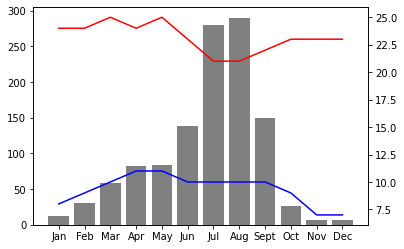
Explanation: in this figure, we put both precipitation data and temperature data (high and low) together. Since several different data records are in the same place, we use the subplots() function to make them appear in one single figure instead of multiple ones. We also choose to add paramaters such as color to differentiate presented data, so that the overall display can convey the information to the readers more effectively.
In summary, first and foremost, any data visualization must accurately and completely reflect the original data. Additionally, scientists should also make a reasonable choice of the data visualization form. In our example of present Addis Ababa’s climate data, we use both a line chart and a histogram to represent a series of data. Both the line chart and the histogram are possible for displaying the differences between any two data points. However, a line chart is usually adopted to reflect the changes whereas a histogram may be more effective to tell the absolute value of data.
We have demonstrated the use of Python’s visualization library, Watplotlib. We must realize that choosing a suitable visualization method is equally as important as choosing a right visualization tool. Furthermore, annotations such as labels and legends are necessary to help people understand the visualization. For making a good data visualization, there are other factors for us to consider, such as chart size, color selections and uses, design styles, animations, and so on.
3.3.6. Exercises#
Exercises
1. An Overview of Data and Data Analysis
Show three different sources of data in the real world and outline the main challenge of analyzing each dataset.
Imagine that a system receives data at 5 Giga Bytes per second (i.e. 5GB/s) for a scientific project. However, the scientists must concurrently process all the data because the store-now-process-later option is unavailable. Moreover, these scientists do not have any single piece of equipment that processes such a large amount of data at that speed. The only systems they have can process 1 GB of data per second (1GB/s). What is your solution to this data processing problem?
Does structured data have higher quality than unstructured data? If so, justify your answer. If not, give a counterexample.
2. Data Operations
Write a Python program that can take a limitless number of user input values but let the program output a maximum of first 6 values. You can freely design and determine how the program takes each value and how it stops accepting user inputs. For example, if the user inputs 1, 2, 3, 4, the program outputs 1, 2, 3, 4. If the user inputs 1, 3, 5, 7, 9, 2, 4, 6, 8, 0, the program outputs 1, 3, 5, 7, 9, 2.
There is a .csv file that stores data like a spreadsheet. There are 100 lines in total. Each line has 25 commas that are used to separate data. This .csv file also contains a title line (in the first row) and an index column (in the first column). The titles and indices are not part of the actual and meaningful data records. Only the remaining fields (i.e. data below the title line and right to the index column) are the actual data records. How many actual data records can this .csv file store?
Assume that an end user inputs a line of data. That line contains all numbers that are separated by comma. For example, the user input from the keyboard is: 150,200,250,300,400,500,50,5,0,1,2 There is a comma (no space) between any two numbers. There is no comma before the first number or after the last number. Write a Python program to read the entire line and parse the data in a way that treats the numbers separately. The program should produce the output with each number in one line, like the following:
150
200
250
300
400
500
50
5
0
1
2
A well-formatted .csv file should have only one kind of data separator, such as commas. What if the original data file contains commas and semicolons both as data separators? Outline a method to correctly process that kind of file.
3. Introduction to Pandas
We will be using the World Population Dataset for this question. The dataset was originally obtained from the World Bank of the United Nations: https://api.worldbank.org/v2/en/indicator/SM.POP.TOTL?downloadformat=csv
Some pre-processing steps have already been taken for the purpose of making this question, including the removal of unnecessary rows from the original file. You can use our prepared file world_population.excel for the data analysis purpose.
a) Read the data file.
A dataset is often so large that we do not want to display everything from it. Sometimes, we just want to take a glance at the structure of the dataset by viewing the first few rows.
b) Display the first 5 rows of data.
Particular rows may be selected for displaying purposes. For example, we may be interested in knowing the population values for a specific country or multiple countries.
c) Display the population values for the country Ethiopia.
d) Select and display all countries and regions whose population is over 10 million in the year of 2000.
Write one Python program that calculates the following values from a given set of numbers: 10301, 4994, 8872, 9624, 3666, 924, 73712, 3823, 55900, 62, 6498, 852, 24540, 421, 67891, 924, 80192, 3667, 494, 1788. You can choose any data structure for the storage and the processing of these numbers. You will then choose and apply any suitable functions for the calculations.
a) the number count, i.e. how many elements in this set.
b) the sum of all these numbers.
c) the minimum value from this set.
d) the maximum value from this set.
e) the median value from this set.
f) the mode of the elements in this set.
g) the standard deviation from this set.
h) the variance (defined as the square of the standard deviation from #7).
4. Basics of matplotlib
If a statistician wants to analyze the data of total births by month in a region, i.e. January: 253, February: 229, March: 247, … What charts would you suggest to use in order to display the monthly records in data visualization? What type of chart is more suitable or less suitable, and for what kind of analysis purpose? Hint: this is a semi-open-ended question. The selection of a chart is determined by a set goal.