10.2. OLS Linear Regression

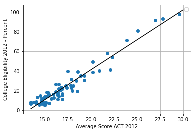
We begin with the familiar topic of ordinary least squares (OLS) linear regression. The table below shows an excerpt of Chicago Public School data for 2011–2012 from the Chicago Data Portal. One expects a higher average ACT score to be associated with a higher percentage of college eligibility.

School zipcode	Average ACT Score	College Eligibility
60605	25.1	80.7
60607	27	91.6
...	...	...
60660	16.5	14.2

Source: Chicago Data Portal,

https://data.cityofchicago.org/Education/Chicago-Public-Schools-Progress-Report-Cards-2011-/9xs2-f89t

The figure below shows a scatterplot of \(n= 83 \) data points partly reproduced in the above table together with the OLS regression line.

10.2.1. Least-Squares Solutions

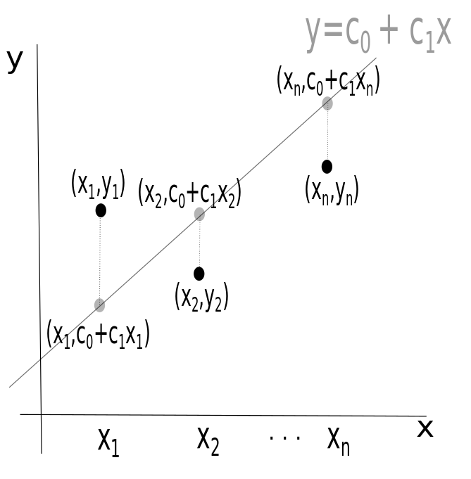
Consider a collection of \(n\) data points \((x_1,y_1),(x_2,y_2),\dots,(x_n,y_n)\) in \(\mathbb{R}^2.\) We seek the line \(y=c_0+c_1x\) that best fits these data, where \(c_0\) is the \(y\)-intercept of the line and \(c_1\) the slope of the line. As shown in the figure below, an OLS loss function \(J(c_0,c_1)\) sums the squared vertical separations between the data points \((x_1,y_1),(x_2,y_2),\dots,(x_n,y_n)\) and the line \(y=c_0+c_1x\).

If the \(n\) data points are collinear, then there exists an exact solution \((c_0,c_1)\) to the system

\[ c_0 + c_1 x_1 = y_1, \]

\[ c_0+c_1x_2 = y_2, \]

\[\vdots\]

\[ c_0+c_1 x_n = y_n. \]

In matrix form, this system of equations becomes

\[ \mathbf{A}\mathbf{c}=\mathbf{y}, \]

where

\[\begin{split} \mathbf{A}= \begin{pmatrix} 1& x_1\\ 1& x_2\\ \vdots&\vdots\\ 1& x_n \end{pmatrix},\quad \mathbf{c}= \begin{pmatrix} c_0\\ c_1 \end{pmatrix}, \quad \, and \, \quad \mathbf{y}= \begin{pmatrix} y_1\\ y_2\\ \vdots\\ y_n \end{pmatrix}. \end{split}\]

In general, this linear system with \(n>2\) equations and 2 unknowns (\(c_0,c_1\)) will not have an exact solution. Instead, our goal to find a linear fit to the data is based on a least-squares solution, one that solves the following optimization problem:

10.2.2. OLS LINEAR REGRESSION OPTIMIZATION PROBLEM

OLS Linear Regression Optimization Problem

Find \((c_0,c_1)\) which minimizes the loss function \(J(c_0,c_1)\) defined as

\[ J(c_0,c_1)=\tfrac{1}{2}\sum_{i=1}^n (y_i-(c_0+c_1x_i) )^2=\tfrac{1}{2}\|\mathbf{y} - \mathbf{A}\mathbf{c}\|^2. \]

(The factor of 1/2 multiplying the sum is introduced to simplify the theoretical analysis of the loss function.)

The loss function \(J\) is zero when the points are collinear and situated on the line \(y=c_0+c_1x\); otherwise, \(J\) is positive, since it is half the sum of the squared vertical separations between data points and the line \(y=c_0+c_1x\), as shown in the previous figure.

10.2.3. Minimizing the OLS Loss Function via Normal Equations

Let \(\mathbf{A}\) be an \(n\times 2\) matrix of real numbers, and let the linear transformation \(\mathbf{L}:\mathbb{R}^2\rightarrow\mathbb{R}^n\) be defined by \(\mathbf{L}(\mathbf{c})= \mathbf{A}\mathbf{c}\), where \(\mathbf{c}\) is a \(2\times 1\) column vector. The range of \(\mathbf{A}\) is the set of all \(n\times 1\) vectors defined by

\[ range\, of \, \mathbf{A} = \{ \mathbf{A}\mathbf{c} \mid \mathbf{c}\in\mathbf{R}^2\}. \]

By choosing \(\mathbf{c}=(1,0)^T\), we see that the first column of \(\mathbf{A}\) (denoted \(\mathbf{a}_1\)) is in the range of \(\mathbf{A}\). By choosing \(\mathbf{c}=(0,1)^T\), we see that the second column of \(\mathbf{A}\) (denoted \(\mathbf{a}_2\)) is also in the range of \(\mathbf{A}\).

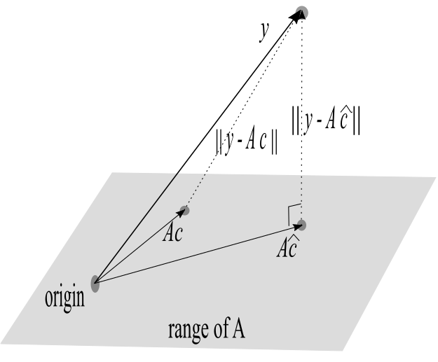
Minimizing the loss function \(J(\mathbf{c}) =\frac{1}{2}\|\mathbf{y} - \mathbf{A}\mathbf{c}\|^2\) is equivalent to minimizing \(\|\mathbf{y} - \mathbf{A}\mathbf{c}\|\), the latter being the distance between \(\mathbf{y}\) and an arbitrary vector \(\mathbf{A} \mathbf{c}\) that is in the range of \(\mathbf{A}\) (see figure below). If there is no exact solution (i.e., \(\mathbf{y}\) is not in the range of \(\mathbf{A})\), this minimization is accomplished by choosing \(\mathbf{\hat{c}}\) such that vector \(\mathbf{y}-\mathbf{A}\hat{c}\) is orthogonal to the range of \(\mathbf{A}\). That is, for \(\mathbf{\hat{c}}\) to be a least-squares solution to \( \mathbf{A}\mathbf{c}=\mathbf{y}\), the vector \(\mathbf{y}-\mathbf{A}\mathbf{\hat{c}}\) must be orthogonal (perpendicular) to each vector in the range of \(\mathbf{A}\). Since both column vectors of \(\mathbf{A}\) (namely, \(\mathbf{a}_1\) and \(\mathbf{a}_2\)) are in the range of \(\mathbf{A}\), it follows that \(\mathbf{a}_i\cdot(\mathbf{y}-\mathbf{A}\mathbf{\hat{c}})=\mathbf{a}_i^T(\mathbf{y}-\mathbf{A}\mathbf{\hat{c}})=0\) for each column vector \(\mathbf{a}_i\) of matrix~\(\mathbf{A}.\)

Hence,

\[ \mathbf{A}^T(\mathbf{y}-\mathbf{A}\mathbf{\hat{c}})=\mathbf{0}\Rightarrow \label{N1} \]

\[ \mathbf{A}^T\mathbf{y}-\mathbf{A}^T\mathbf{A}\mathbf{\hat{c}} = \mathbf{0}\Rightarrow \]

\[ \mathbf{A}^T\mathbf{y}=\mathbf{A}^T\mathbf{A}\mathbf{\hat{c}} \]

The last equation is called the normal equation for the system \(\mathbf{A}\mathbf{c}=\mathbf{y}.\) Solving the normal equations, one obtains optimal values for \(c_0,c_1\).

Example 2.1.

Example 2.1

Consider the data \((-1, 1)\), \((0, 0)\), \((1, 2)\), \((2, 3)\). Use the normal equations to find the OLS regression line for the data.

Solution.

The system is

\[\begin{align*} c_0-c_1&=1,\\ c_0&=0,\\ c_0+c_1&=2,\\ c_0+2c_1&=3;\\ \end{align*}\]

or, in matrix form,

\[\begin{align*} \begin{pmatrix} 1& -1\\ 1& 0\\ 1&1\\ 1& 2 \end{pmatrix} \begin{pmatrix} c_0\\ c_1 \end{pmatrix}= \begin{pmatrix} 1\\ 0\\ 2\\ 3 \end{pmatrix}. \end{align*}\]

The normal equations are

(10.1)\[\begin{eqnarray} \begin{pmatrix} 1& 1&1&1\\ -1&0&1&2 \end{pmatrix} \begin{pmatrix} 1\\ 0\\ 2\\ 3 \end{pmatrix}= \begin{pmatrix} 1& 1&1&1\\ -1&0&1&2 \end{pmatrix} \begin{pmatrix} 1& -1\\ 1& 0\\ 1&1\\ 1& 2 \end{pmatrix} \begin{pmatrix} c_0\\ c_1 \end{pmatrix}, \label{ne} \end{eqnarray}\]

or

\[\begin{eqnarray*} \begin{pmatrix} 6\\ 7 \end{pmatrix}= \begin{pmatrix} 4&2\\ 2&6 \end{pmatrix} \begin{pmatrix} c_0\\ c_1 \end{pmatrix}. \end{eqnarray*}\]

The least-squares solution is therefore \(c_0=11/10\), \(c_1=4/5.\)

10.2.4. Equivalence of Gradient-Based Optimization

Note that the normal equations are equivalent to gradient-based minimization of the OLS linear regression loss function \(J(c_0,c_1)=\frac{1}{2}\sum_{i=1}^n (y_i-(c_0+c_1x_i) )^2\):

\[\begin{align*} \mathbf{A}^T(\mathbf{y}-\mathbf{A}\mathbf{\hat{c}})&= \begin{pmatrix} 1 & 1& \dots& 1\\ x_1&x_2&\dots&x_n \end{pmatrix} \begin{pmatrix} y_1-(c_0+c_1x_1)\\ y_2-(c_0+c_1x_2)\\ \dots\\ y_n-(c_0+c_1x_n) \end{pmatrix}\\ &= \begin{pmatrix} \sum_{i=1}^n \bigl(y_i-(c_0+c_1x_i)\bigr)\\\\ \sum_{i=1}^n x_i\bigl(y_i-(c_0+c_1x_i)\bigr) \end{pmatrix}= \begin{pmatrix} -\tfrac{\partial J}{\partial c_0}\\ -\tfrac{\partial J}{\partial c_1} \end{pmatrix}= \begin{pmatrix} 0\\ 0 \end{pmatrix}. \end{align*}\]

The normal equations are equivalent to setting both partial derivatives of \(J\) equal to zero, as is required to minimize the loss function \(J(c_0,c_1)\).

Example 2.2.

Example 2.2

For the data points in Example 2.1, show how gradient-based optimization of the loss function \(J\) gives the same values for \(c_0\) and \(c_1\).

Solution:

The loss function \(J(c_0,c_1)\) is

\[\begin{align*} J(c_0,c_1)&=\tfrac{1}{2}[\bigl(1-(c_0-c_1)\bigr)^2+(0-c_0)^2+\bigl(2-(c_0+c_1)\bigr)^2+\\ &\qquad\bigl(3-(c_0+2c_1)\bigr)^2]. \end{align*}\]

To minimize \(J\), we solve the linear system for \(\nabla J(c_1,c_2)=\mathbf{0}\):

\[ \frac{\partial J}{\partial c_0} =4c_0+2c_1-6=0, \qquad \frac{\partial J}{\partial c_1} =2c_0+6c_1-7=0. \]

Solving this system, we obtain \(c_0=11/10\) and \(c_1=4/5\).

The system used to find these critical values is equivalent to:

(10.2)\[\begin{align} %\scriptstyle \begin{pmatrix} %\scriptstyle -\frac{\partial J}{\partial c_0}\\ -\frac{\partial J}{\partial c_1} \end{pmatrix}&= \begin{pmatrix} \scriptstyle \bigl(1-(c_0-c_1)\bigr)+(0-c_0)+\bigl(2-(c_0+c_1)\bigr)+\bigl(3-(c_0+2c_1\bigr) \\ \scriptstyle-\bigl(1-(c_0-c_1)\bigr)+0(0-c_0)+\bigl(2-(c_0+c_1)\bigr)+2\bigl(3-(c_0+2c_1)\bigr) \end{pmatrix}\nonumber\\ &= \scriptstyle\begin{pmatrix} 1& 1&1&1\\ -1&0&1&2 \end{pmatrix} \scriptstyle \begin{pmatrix} 1\\ \textstyle 0\\ 2\\ 3 \end{pmatrix}- \scriptstyle\begin{pmatrix} 1& 1&1&1\\ -1&0&1&2 \end{pmatrix} \scriptstyle\begin{pmatrix} 1& -1\\ 1& 0\\ 1&1\\ 1& 2 \end{pmatrix} \scriptstyle\begin{pmatrix} c_0\\ c_1 \end{pmatrix}= \scriptstyle \begin{pmatrix} 0\\ 0 \end{pmatrix}, \label{ne1} \end{align}\]

Gradient-based optimization expressed is indeed equivalent to the normal equations.

To say that solving the normal equations is mathematically equivalent to gradient-based optimization of the OLS loss function does not imply that the normal equations offer the best numerical method for optimization of the loss function [Epperly 2022]. Beyond the scope of this Module is an assessment of different numerical approaches such as gradient descent and its variants including the Adam method [Sun et. al. 2019], matrix factorizations such as \(SVD\) or \(QR\) [Aggarwal 2020], and mean-centering and standardizing data [Toth 2020].

In addition to facilitating numerical analysis, mean-centering simplifies the linear algebra approach. Mean-centered data is obtained from a collection of data points by replacing the original dataset \((x_i,y_i)\) with the data points \((x_i-\bar{x},y_i-\bar{y})\), \(i=1, \dots n\), where \(\bar{x}\) and \(\bar{y}\) are the respective means of the \(x\) and \(y\) coordinates of the original data. One can show that for mean-centered data, \(\hat{c}_0=0\), and the regression line is \(y = \hat{c}_1 x\). Let \(\mathbf{x}=(x_1,x_2,...,x_n)^{tr}\). For mean-centered data, the regression vector \({\bf \hat{y}}=\hat{c}_1\mathbf{x}\) is obtained by projecting the vector \({\bf y}\) directly onto the vector \({\bf x}\) as shown in the figure below.

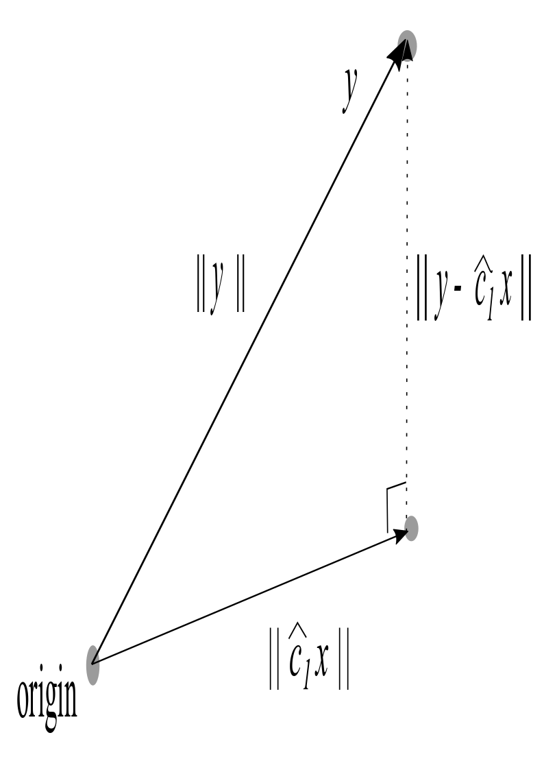
The variation equation states that the total variation in the y-values is the sum of the explained variation (variation in the corresponding \(y\)-values on the regression line) and the unexplained variation (the sum of squared residuals or twice the value of the loss function \(J\)). For mean-centered data, the total variation is \(\mid\mid \mathbf{y}\mid\mid^2\), the explained variation is \(\mid\mid \hat{c}_1\mathbf{x}\mid\mid^2\) and the unexplained variation is \(\mid\mid \mathbf{y} -\hat{c}_1 \mathbf{x}\mid\mid^2\). In other words, the variation equation for mean-centered data is simply the Pythagorean theorem.

10.2.5. Practice Problems

Practice Problems

1. Consider the data \((1, 0)\), \((4, 5)\), \((7, 8)\). Use the normal equations to find the least-squares solution line \(y = a + bx\) that best fits the data.

2. Consider the data \((-1,1)\), \((0,0)\), \((1,2)\), \((2,3)\). Use the normal equations to find the least-squares solution for the parabola \(y=a+bx+cx^2\) that best fits the data.

Solutions to Practice Problems

Problem 1) The system is

\[\begin{align*} a+b&=0,\\ a + 4b&=5,\\ a+7b&=8; \end{align*}\]

or, in matrix form,

\[\begin{align*} \begin{pmatrix} 1& 1\\ 1& 4\\ 1&7\\ \end{pmatrix} \begin{pmatrix} a\\ b\\ \end{pmatrix}= \begin{pmatrix} 0\\ 5\\ 8\\ \end{pmatrix}. \end{align*}\]

The normal equations are

\[\begin{align*} \begin{pmatrix} 1& 1&1\\ 1&4&7\\ \end{pmatrix} \begin{pmatrix} 0\\ 5\\ 8\\ \end{pmatrix}= \begin{pmatrix} 1& 1&1\\ 1&4&7\\ \end{pmatrix} \begin{pmatrix} 1& 1\\ 1& 4\\ 1&7\\ \end{pmatrix} \begin{pmatrix} a\\ b \end{pmatrix}, \end{align*}\]

or

\[\begin{align*} \begin{pmatrix} 13\\ 76 \end{pmatrix}= \begin{pmatrix} 3&12\\ 12&66 \end{pmatrix} \begin{pmatrix} a\\ b \end{pmatrix}. \end{align*}\]

Solving the normal equations gives the least-squares solution \(a=-1\), \(b=4/3\).

Problem 2)

The system is

\[\begin{align*} a-b+c&=1,\\ a&=0,\\ a+b+c&=2,\\ a+2b+4c&=3;\\ \end{align*}\]

or, in matrix form,

\[\begin{align*} \begin{pmatrix} 1& -1&1\\ 1& 0&0\\ 1&1&1\\ 1& 2&4 \end{pmatrix} \begin{pmatrix} a\\ b\\ c \end{pmatrix}= \begin{pmatrix} 1\\ 0\\ 2\\ 3 \end{pmatrix}. \end{align*}\]

The normal equations are

\[\begin{align*} \begin{pmatrix} 1& 1&1&1\\ -1&0&1&2\\ 1&0&1&4 \end{pmatrix} \begin{pmatrix} 1\\ 0\\ 2\\ 3 \end{pmatrix}= \begin{pmatrix} 1& 1&1&1\\ -1&0&1&2\\ 1&0&1&4 \end{pmatrix} \begin{pmatrix} 1& -1&1\\ 1& 0&0\\ 1&1&1\\ 1& 2&4 \end{pmatrix} \begin{pmatrix} a\\ b \end{pmatrix}, \end{align*}\]

or

\[\begin{align*} \begin{pmatrix} 6\\ 7\\ 15 \end{pmatrix}= \begin{pmatrix} 4&2&6\\ 2&6&8\\ 6&8&18 \end{pmatrix} \begin{pmatrix} a\\ b\\ c \end{pmatrix}. \end{align*}\]

Solving the normal equations gives the least-squares solution \(a=3/5, b=3/10\), and \(c=1/2.\)

10.2.6. Lab

In this lab we will make scatterplots of data which include the OLS regression line.

We begin by importing libraries.

import numpy as np
import pandas as pd
import matplotlib.pyplot as plt
from sklearn.linear_model import LinearRegression

Example 1

OLS Regression of ACT and College Eligibility

Datafile: ACTCollegeEligible.csv

1. Import Libraries, dropping rows with missing data.

df=pd.read_csv("ACTCollegeEligible.csv")
df=df.dropna()
df.head(2)

	School Name	Street Address	ZIP	Average Score ACT 2012	5-Year Cohort Graduation Rate 2012 - Percent	One-Year Dropout Rate 2012 - Percent	Freshman On-Track to Graduate 2012 - Percent	College Eligibility 2012 - Percent	College Enrollment 2012 - Percent	College Retention 2010 - Percent	Misconducts Resulting in Suspensions 2012 - Percent	Average Days of Suspension 2012	Student Attendance 2012 - Percent	Teacher Attendance 2012 - Percent	X Coordinate	Y Coordinate	Longitude	Latitude	Location
0	Chicago Academy High School	3400 N Austin Ave	60634	19.3	71.0	4.0	82.2	35.2	75.8	71.0	4.5	2.6	93.6	95.6	1135740.091	1922002.941	-87.776506	41.942154	(-87.77650575, 41.94215439)
3	William Jones College Preparatory High School	606 S State St	60605	25.1	87.1	1.5	98.0	80.7	92.2	90.8	10.6	4.5	93.9	95.3	1176412.354	1897618.088	-87.627755	41.874419	(-87.62775497, 41.87441898)

2. Specify the x and y coordinates of the points to be plotted.

X=df[["Average Score ACT 2012"]]
Y=df[["College Eligibility 2012 - Percent"]]

3. Create the OLS regression model.

OLSmodel = LinearRegression()
OLSmodel.fit(X, Y)
print("OLS regression line y=mx+b")
print("slope m=",OLSmodel.coef_)
print("intercept b=",OLSmodel.intercept_)

OLS regression line y=mx+b
slope m= [[6.09611136]]
intercept b= [-80.78259412]

4. Make the scatterplot with regression line.

from sklearn.linear_model import LinearRegression #sklearn is a machine learning library
X=df[["Average Score ACT 2012"]]
Y=df[["College Eligibility 2012 - Percent"]]
reg=LinearRegression()
reg.fit(X,Y)
print("Intercept is ", reg.intercept_)
print("Slope is ", reg.coef_)
print("R^2 for OLS is ", reg.score(X,Y))
# x values on the regression line will be between 13.5 and 30 
x = np.linspace(13.5, 30 ,100) 
# define the regression line y = mx+b here
[[m]]=reg.coef_
[b]=reg.intercept_
y =  m*x  + b   
#plot the data points 
fig=df.plot(x="Average Score ACT 2012", y="College Eligibility 2012 - Percent", style='o')  
plt.xlabel("Average Score ACT 2012")  
plt.ylabel("College Eligibility 2012 - Percent")  
# plot the regression line 
plt.plot(x,y, 'k') #add the color for red
plt.legend([],[], frameon=True)
plt.grid()
plt.show()

Intercept is  [-80.78259412]
Slope is  [[6.09611136]]
R^2 for OLS is  0.9351396968249491

Example 2

Linear Regression of Chicago Public School Data

Data File: Imported directly from the Chicago data portal in Step 1.

1. Let’s begin by executing the following cell to retrieve a Chicago Public School (CPS) dataset.

import pandas as pd
import numpy as np
raw_CPS_data=  pd.read_json('https://data.cityofchicago.org/resource/kh4r-387c.json?$limit=100000')
raw_CPS_data.head() 

	school_id	legacy_unit_id	finance_id	short_name	long_name	primary_category	is_high_school	is_middle_school	is_elementary_school	is_pre_school	...	fifth_contact_title	fifth_contact_name	seventh_contact_title	seventh_contact_name	refugee_services	visual_impairments	freshman_start_end_time	sixth_contact_title	sixth_contact_name	hard_of_hearing
0	609966	3750	23531	HAMMOND	Charles G Hammond Elementary School	ES	False	True	True	True	...	NaN	NaN	NaN	NaN	NaN	NaN	NaN	NaN	NaN	NaN
1	400069	4150	67081	POLARIS	Polaris Charter Academy	ES	False	True	True	False	...	NaN	NaN	NaN	NaN	NaN	NaN	NaN	NaN	NaN	NaN
2	610191	6070	29291	STONE	Stone Elementary Scholastic Academy	ES	False	True	True	False	...	NaN	NaN	NaN	NaN	NaN	NaN	NaN	NaN	NaN	NaN
3	400173	9648	66801	PATHWAYS - BRIGHTON PARK HS	Pathways in Education- Brighton Park	HS	True	False	False	False	...	NaN	NaN	NaN	NaN	NaN	NaN	NaN	NaN	NaN	NaN
4	610153	5670	25191	RYDER	William H Ryder Math & Science Specialty ES	ES	False	True	True	True	...	NaN	NaN	NaN	NaN	NaN	NaN	NaN	NaN	NaN	NaN

5 rows × 92 columns

2. Let’s get the column names

raw_CPS_data.columns

Index(['school_id', 'legacy_unit_id', 'finance_id', 'short_name', 'long_name',
       'primary_category', 'is_high_school', 'is_middle_school',
       'is_elementary_school', 'is_pre_school', 'summary',
       'administrator_title', 'administrator', 'secondary_contact_title',
       'secondary_contact', 'address', 'city', 'state', 'zip', 'phone', 'fax',
       'cps_school_profile', 'website', 'facebook', 'attendance_boundaries',
       'grades_offered_all', 'grades_offered', 'student_count_total',
       'student_count_low_income', 'student_count_special_ed',
       'student_count_english_learners', 'student_count_black',
       'student_count_hispanic', 'student_count_white', 'student_count_asian',
       'student_count_native_american', 'student_count_other_ethnicity',
       'student_count_asian_pacific', 'student_count_multi',
       'student_count_hawaiian_pacific', 'student_count_ethnicity_not',
       'statistics_description', 'demographic_description', 'dress_code',
       'prek_school_day', 'kindergarten_school_day', 'school_hours',
       'after_school_hours', 'earliest_drop_off_time', 'classroom_languages',
       'bilingual_services', 'title_1_eligible', 'preschool_inclusive',
       'preschool_instructional', 'transportation_bus', 'transportation_el',
       'school_latitude', 'school_longitude', 'overall_rating',
       'rating_status', 'rating_statement', 'classification_description',
       'school_year', 'third_contact_title', 'third_contact_name', 'network',
       'is_gocps_participant', 'is_gocps_prek', 'is_gocps_elementary',
       'is_gocps_high_school', 'open_for_enrollment_date', 'twitter',
       'youtube', 'pinterest', 'college_enrollment_rate_school',
       'college_enrollment_rate_mean', 'graduation_rate_school',
       'graduation_rate_mean', 'significantly_modified',
       'transportation_metra', 'fourth_contact_title', 'fourth_contact_name',
       'fifth_contact_title', 'fifth_contact_name', 'seventh_contact_title',
       'seventh_contact_name', 'refugee_services', 'visual_impairments',
       'freshman_start_end_time', 'sixth_contact_title', 'sixth_contact_name',
       'hard_of_hearing'],
      dtype='object')

3. Let’s find the number of rows in each column which have data using a command of the form df.count().

raw_CPS_data.count()

school_id                  654
legacy_unit_id             654
finance_id                 654
short_name                 654
long_name                  654
                          ... 
visual_impairments           6
freshman_start_end_time    101
sixth_contact_title         45
sixth_contact_name          45
hard_of_hearing             13
Length: 92, dtype: int64

4. Let’s check what entries there are in the ‘grades_offered’ column.

raw_CPS_data['grades_offered'].value_counts()

grades_offered
PK,K-8       327
9-12         144
K-8           82
7-12          11
PK,K-6        10
PK,K-5        10
6-12           9
K-6            8
6-8            6
PK,K-4         4
K-12           4
PE,PK,K-8      4
11-12          4
5-8            3
PK             3
K-5            3
PK,K-3         3
8-12           2
PK,K-2         2
7-8            2
PK,3-8         1
9              1
K,4-8          1
K-1,5-8        1
3-12           1
K-3,5-8        1
1-8            1
PK,K-7         1
10-12          1
4-11           1
K-3            1
K-2            1
4-8            1
Name: count, dtype: int64

5. Let’s create a dataframe called mid with just the data for PK,K-8

mid=raw_CPS_data[raw_CPS_data['grades_offered']=='PK,K-8']
mid.head(2)

	school_id	legacy_unit_id	finance_id	short_name	long_name	primary_category	is_high_school	is_middle_school	is_elementary_school	is_pre_school	...	fifth_contact_title	fifth_contact_name	seventh_contact_title	seventh_contact_name	refugee_services	visual_impairments	freshman_start_end_time	sixth_contact_title	sixth_contact_name	hard_of_hearing
0	609966	3750	23531	HAMMOND	Charles G Hammond Elementary School	ES	False	True	True	True	...	NaN	NaN	NaN	NaN	NaN	NaN	NaN	NaN	NaN	NaN
4	610153	5670	25191	RYDER	William H Ryder Math & Science Specialty ES	ES	False	True	True	True	...	NaN	NaN	NaN	NaN	NaN	NaN	NaN	NaN	NaN	NaN

2 rows × 92 columns

6. Let’s streamline the data to a dataframe df which includes just the columns [‘address’,‘student_count_total’,‘student_count_black’,‘student_count_hispanic’,‘student_count_white’,‘zip’]

df=raw_CPS_data[['address','student_count_total','student_count_black','student_count_hispanic','student_count_white','zip']]
df.head(2)

	address	student_count_total	student_count_black	student_count_hispanic	student_count_white	zip
0	2819 W 21ST PL	342	33	304	2	60623
1	620 N SAWYER AVE	378	337	33	5	60624

7. Let’s get all the schools with zip 60623

df23=df[df['zip']==60623]
df23.head(2)

	address	student_count_total	student_count_black	student_count_hispanic	student_count_white	zip
0	2819 W 21ST PL	342	33	304	2	60623
11	2345 S CHRISTIANA AVE	559	66	484	9	60623

7. Let’s reset the index.

df23=df23.reset_index(drop=True)
df23.head(5)

	address	student_count_total	student_count_black	student_count_hispanic	student_count_white	zip
0	2819 W 21ST PL	342	33	304	2	60623
1	2345 S CHRISTIANA AVE	559	66	484	9	60623
2	3500 W DOUGLAS BLVD	216	212	4	0	60623
3	3711 W DOUGLAS BLVD	499	480	14	3	60623
4	4217 W 18TH ST	316	306	10	0	60623

8. What is the size of the biggest CPS PK,K-8 in 60623?

max=df23["student_count_total"].max()
max

1072

9. What is the size of the smallest CPS PK,K-8 in 60623?

min=df23["student_count_total"].min()
min

96

10. Let’s simplify the column names to [“address”,“total”,“black”,“hispanic”,“white”]

df23.columns= ["address","total","black","hispanic","white","zip"]
df23.head(1)

	address	total	black	hispanic	white	zip
0	2819 W 21ST PL	342	33	304	2	60623

10. Let’s create 3 new columns ‘%black’, ‘%hispanic’, ‘%white’

for i in df23.index:
    df23.loc[i,'%black']=round(100*df23.loc[i,'black']/df23.loc[i,'total'],1)
    df23.loc[i,'%hispanic']=round(100*df23.loc[i,'hispanic']/df23.loc[i,'total'],1)
    df23.loc[i,'%white']=round(df23.loc[i,'white']/df23.loc[i,'total'],1)
df23.head(5)

	address	total	black	hispanic	white	zip	%black	%hispanic	%white
0	2819 W 21ST PL	342	33	304	2	60623	9.6	88.9	0.0
1	2345 S CHRISTIANA AVE	559	66	484	9	60623	11.8	86.6	0.0
2	3500 W DOUGLAS BLVD	216	212	4	0	60623	98.1	1.9	0.0
3	3711 W DOUGLAS BLVD	499	480	14	3	60623	96.2	2.8	0.0
4	4217 W 18TH ST	316	306	10	0	60623	96.8	3.2	0.0

Exercise

Exercise

Make a scatterplot which shows the %black (x-axis) vs. %hispanic (y-axis) and include the OLS regression line on the plot. What does the graph tell us about grade pre K - 8 schools in Chicago zip code 60623?

The graph show that schools are predominantly hispanic or predominantly black.