Show code cell source Hide code cell source

import numpy as np
import matplotlib.pyplot as plt
import math
%matplotlib inline

7.13. Ordinary Differential Equations and Exponential Growth/Decay

Simply put, a differential equation is an equation that includes at least one derivative of a function. For example,

\[ \frac{dy}{dt} = y, \]

is a differential equation involving a function \(y(t)\) and its first derivative \(\frac{dy}{dt}\).

Differential equations are used widely across many areas of science, economics, and mathematics.

7.13.1. Initial Value Problems

An initial value problem (IVP) consists of a differential equation (DE) and an initial condition (IC). Here is an example:

\[ (DE)\, \frac{dy}{dt} = \frac{1}{y}, \]

\[ (IC)\, y(0) =1 \]

7.13.2. Separation of Variables

A basic technique which can be used to solve simple IVP’s is called separation of variables. Here is how we solve the above IVP using this technique:

1. bring to one side of the equation all the \(y\)’s times \(dy\), and to the other side of the equation all the \(t's\) times \(dt\):

\[ y\,dy = \, \, dt. \]

2. Integrate both sides of the equation:

\[ \int y\,dy = \, \int \, dt \Rightarrow \frac{y^2}{2} = t + C. \]

3. Use the initial condition (IC) \(y(0)=1\) (i.e. \(y=1\) when \(t=0\)) to find the value of \(C\):

\[ \frac{1}{2}= 0 + C \Rightarrow C=\frac{1}{2}. \]

4. Substitute the value for \(C\).

\[ \frac{y^2}{2} = t + \frac{1}{2}. \]

5. Solve for \(y\).

\[ y^2 = 2t + 1. \]

\[ y=\sqrt{2t+1} . \]

Note that we use the positive square root to satisfy the IC \(y(0)=1\).

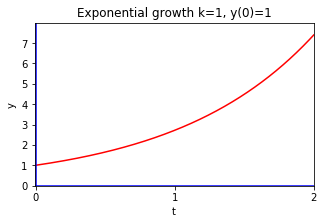
7.13.3. Exponential Growth

In some situations such as continuous compounding of interest, the rate of growth of a quantity is proportional to the size of the quantity:

\[ \frac{dy}{dt} = k y. \]

The constant \(k>0\) is called the growth constant.

If at \(t=0\) the value of \(y\) is \(y_0\) (that is we are given the IC: \(y(0)=y_0\)), we can use separation of variables to solve for \(y(t)\):

\[ \frac{dy}{y} = k dt \]

\[ \int \frac{dy}{y} = k \int dt \]

\[\ln(y) = kt+C \]

\[ y = e^{kt+c}=e^{kt}e^C = C_1 e^{kt}\]

\[ y(0) = C_1 e^0 = C_1 = y_0.\]

Thus, our solution is \(y(t)=y_0 e^t.\)

Show code cell source Hide code cell source

f = lambda t : y0 * np.exp(t)
y0=1
plt.figure(figsize=(5,3))
t=np.arange(0,2.1,.001)
y=f(t)
plt.gca().set_xticks(np.arange(0,2.1))
plt.gca().set_yticks(np.arange(0,8,1))
plt.plot(t,y,'r',markersize=1)
plt.title('Exponential growth k=1, y(0)=1')
plt.xlabel('t')
plt.ylabel('y')
plt.xlim((-.01,2)) 
plt.ylim((-.01,8))
plt.gca().axhline(y=0, color='b')
plt.gca().axvline(x=0, color='b')
plt.savefig('expgrowth.png')
plt.show()

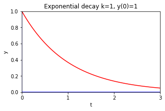
7.13.4. Exponential Decay

In some situations such as radioactive decay, the IVP is

\[\frac{dy}{dt} = - ky, \,y(0)=y_0. \]

Using separation variables in a similar way to solving the exponential growth equation leads to the solution

\[y(t)=y_0 e^{-kt}. \]

Show code cell source Hide code cell source

f = lambda t : y0 * np.exp(-t)
y0=1
plt.figure(figsize=(5,3))
t=np.arange(0,3.1,.001)
y=f(t)
plt.gca().set_xticks(np.arange(0,3.1))
plt.gca().set_yticks(np.arange(0,1.1,.2))
plt.plot(t,y,'r',markersize=1)
plt.title('Exponential decay k=1, y(0)=1')
plt.xlabel('t')
plt.ylabel('y')
plt.xlim((0,3)) 
plt.ylim((0,1))
plt.gca().axhline(y=0, color='b')
plt.gca().axvline(x=0, color='b')
plt.savefig('expdecay.png')
plt.show()

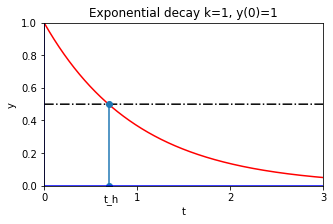
Half-Life

For radioactive decay problems, the time it takes for radioactive material to decay to half the original amount is called the half-life.

To find the half-life \(t=t_h\) for the case \(k=1\), we solve as follows:

\[ y(t_h)= y_0 e^{-t_h}=\frac{1}{2}y_0\]

\[e^{-t_h}=\frac{1}{2}\]

\[-t_h=\ln\frac{1}{2}\]

\[t_h=-\ln\frac{1}{2} = \ln 2\approx .69. \]

Show code cell source Hide code cell source

f = lambda t : y0 * np.exp(-t)
y0=1
plt.figure(figsize=(5,3))
t=np.arange(0,3.1,.001)
y=f(t)
plt.gca().set_xticks(np.arange(0,3.1))
plt.gca().set_yticks(np.arange(0,1.1,.2))
plt.plot(t,y,'r',markersize=1)
plt.plot(t,0*t+.5,'-.k')
plt.title('Exponential decay k=1, y(0)=1')
x1, y1 = [np.log(2),np.log(2)], [0,.5]
plt.plot(x1, y1,marker = 'o')
plt.xlabel('t')
plt.ylabel('y')
plt.xlim((0,3)) 
plt.ylim((-.001,1))
plt.gca().axhline(y=0, color='b')
plt.gca().axvline(x=0, color='b')
plt.text(.64,-.1,'t_h')
plt.savefig('expdecay.png')
plt.show()

7.13.5. Exercises

Exercises

1. Let \(y(t)\) be the amount (in grams) of a pollutant at time \(t\) (in days) found in a certain water supply. Suppose after an industrial accident, \(y(0)=100\) and additional pollutant enters the water supply at a constant rate of \(c_1= 5\) gm/day. Emergency water purification measures are used to reduce the daily amount of pollutant at a rate of 1% of the existing amount of pollution.

a) What IVP is used to model this situation?

Hint: The rate of change of pollutant \(\frac{dy}{dt}\) is equal to rate in - rate out.

b) Use separation of variables to solve the IVP.

c) Suppose the water supply becomes unsafe if the pollution level reaches 400 gm. After how many days will the water supply become unsafe?

d) Make a graph of \(y(t)\).

2. Prove the Rule of 72: If money is deposited into an account with an annual interest rate \(r\) (expressed as a percentage) compounded continuously, then it will take roughly \(72/r\) years for the money to double.

3. For exponential decay, find a formula relating the decay constant \(k\) and the half-life \(t_h\).

4. The exponential growth model predicts that \(y\rightarrow\infty\) as \(t\rightarrow\infty.\) This may not be realistic. For example, if \(y(t)\) represents the population at time \(t\), there is a limit to how big \(y(t)\) can grow.

The logistic model includes a cap \(M\) on how big the population can grow, and is given by the following IVP:

\[ \frac{dy}{dt} = ky(M-y),\,y(0)=y_0. \]

Use separation of variables to solve the logistic growth model for the case \(k=1\), \(M=100\), \(y_0=5\).

Hint:

\[ \frac{1}{y(M-y)}=\frac{1}{M}(\frac{1}{y}+\frac{1}{M-y}). \]