Show code cell source
import pandas as pd
import numpy as np
import matplotlib.pyplot as plt
7.3. Marginal and Average Cost#
7.3.1. Derivative Rules#
Given a function \(y=f(x)\), the derivative \(f'(x)\) evaluated at \(x=a\) gives the slope of the tangent to the graph of \(y=f(x)\) at the point \((a,f(a))\).
There are rules to quickly finding the derivative of polynomials and functions with powers.
If \(f(x)=mx+b\), then \(f'(x)=m.\)
If \(f(x)=kx^n,\) then \(f'(x)=knx^{n-1}.\)
If \(f(x)=a_0+a_1x+a_2x^2+a_3x^3\), then \(f'(x)=a_1+2a_2x + 3a_3 x^2\).
(Note that the derivative of the constant term by itself is 0. The same pattern continues for higher powers).
EXAMPLE: If \(f(x)=2x^3 -5x^2+2x + 10\), then \(f'(x)=6x^2-10x+2.\)
EXAMPLE: If \(f(x)=\frac{2}{\sqrt{x}}=2x^{-.5}\), then \(f'(x)=2(-.5)x^{-1.5}=\frac{-1}{x^{1.5}}\)
7.3.2. Marginal Functions#
The term ``marginal’’ is used to mean derivative.
EXAMPLE: Let TC be total cost and Q be the number of units produced. If \(TC(Q)= 50+10 Q^{3/2}\), then the marginal cost is \(MC(Q)=TC'(Q)=10(3/2) Q^{1/2}=15\sqrt{Q}\)
Note: Since the derivative of a function \(f(x)\) is given by
if we choose \(h=1\), then we get an approximation
Thus, marginal functions can be used to approximate the difference between the value of the original function at \(x+1\) and the value of the original function at \(x\).
For the total cost function, the derivative \(MC(Q)=TC'(Q)\) approximates the difference in total cost producing \(Q+1\) units and producing \(Q\) units. In other words, the marginal total cost approximates the the total cost to produce 1 more unit if the current production level is \(Q\).
7.3.3. Fixed Cost#
The term ``fixed cost’’ means the cost incurred when \(Q=0\) units are produced.
EXAMPLE: Let \(TC(Q)=50+10 Q^{3/2}. \) Then the fixed cost is \(TC(0)=50.\)
7.3.4. Demand Function#
A demand function \(P(Q)\) gives the price \(P\) per unit when selling \(Q\) units. The total revenue \(TR\) generated by selling \(Q\) units is therefore \(TR=Q \cdot P(Q).\)
Example 1. Find the total revenue \(TR\) and marginal revenue \(MR\) if the demand function is \(P=100-5\sqrt{Q}\).
Answer: \(TR=Q(100-5\sqrt{Q})=100Q - 5Q\sqrt{Q}=100Q-5Q(Q^{.5})=100Q-5Q^{1.5}\).
\(MR=TR'=100-5(1.5)Q^{.5}=100-7.5Q^{.5}.\)
Example 2. Algebra might be needed to find the demand function \(P(Q)\).
If \(Q=\frac{10}{P^2}\), then \(P^2=\frac{10}{Q}\Rightarrow P=\frac{\sqrt{10}}{\sqrt{Q}}.\) The total revenue is therefore \(TR= Q\cdot P = Q (\frac{\sqrt{10}}{\sqrt{Q}}) = \sqrt{Q} \sqrt{10} = \sqrt{10}Q^{1/2}.\) It follows that the marginal revenue is \(MR=\frac{1}{2}\sqrt{10}Q^{-1/2}= \frac{\sqrt{10}}{2\sqrt{Q}}\).
7.3.5. Average Cost#
The average cost equals the total cost divided by number of units produced.
EXAMPLE. If the total cost is \(TC= 10Q^2+ 5Q+10,\) then the average cost is \(AC=\frac{TQ}{Q}=10Q + 5 + \frac{10}{Q}\)
7.3.6. Graphical Intersections#
To find a point where the graph of \(f(x)\) intersects the graph of \(g(x)\), solve the equation \(f(x)=g(x).\) (For our applications we require that \(x\ge 0\))
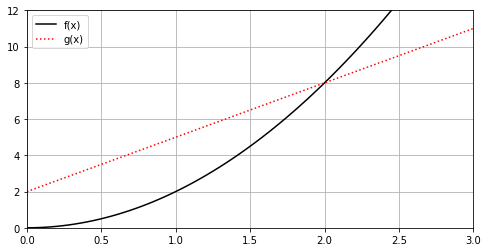
EXAMPLE: Find where \(f(x)=2x^2\) and \(g(x)=3x+2\) intersect.
Solution. We must solve \(2x^2=3x+2\). That is \(2x^2-3x-2=0\). To solve \(ax^2+bx+c=0,\) we can use the quadratic formula \(x=\frac{-b\pm \sqrt{b^2-4ac}}{2a}.\) In our case,
(We do not use the other root at \(x= -1/2\) since we require \(x\ge 0\)).
The \(y\)-coordinate of the intersection point with \(x=2\) is \(y=f(2)=2(2^2)=8\). Note that \(g(2)=3(2)+2=8\) so in fact, the graph of both \(f(x)\) and \(g(x)\) includes the point \((2,8)\)
Show code cell source
x = np.linspace(0,4,100)
f= 2*x**2  #first function
g=3*x+2 # second function
plt.figure(figsize=(8, 4))
plt.plot(x,f,color='k',label="f(x)")
plt.plot(x,g,color='r',linestyle=":",label="g(x)")
plt.xlim((0.,3))
plt.ylim((0,12.))
plt.grid()
plt.legend()
plt.show()
7.3.7. Exercises#
Exercises
Consider the total cost function
Find and graph the average total cost \(ATC\) and the marginal cost \(MC\). Use the graph to determine where \(ATC=MQ\). Then show that \(ATC\) has a minimum value at the point of intersection. (That is, show that \(ATC'(Q)=0\) at the point of intersection).
Repeat problem 1 using the total cost function
(In this case, the average total cost has a maximum rather than minimum value at the point of intersection.)
The quotient rule says that
Use the quotient rule to prove that the average total cost must have a max or min at the point where it equals the marginal cost.