12.5. CWS Model of Alzheimer’s Disease#
Acknowledgements
This material was published previously in an article in the UMAP Journal titled The CWS Model of Alzheimer’s Disease. The UMAP Journal 34(1) (2013) 3-18. Copyright 2021 by COMAP, Inc. All rights reserved. Author: Paul Isihara with Anne Bowen, Isaac Brown, Tim Dennison,Wesley Hanna, and Kyle Williams. Permission to make digital or hard copies of part or all of this work for personal or classroom useis granted without fee provided that copies are not made or distributed for profit or commercial advantage and that copies bear this notice. Abstracting with credit is permitted, but copyrights for components of this work owned by others than COMAP must be honored. To copy otherwise, to republish, to post on servers, or to redistribute to lists requires prior permission from COMAP.
12.5.1. Introduction#
The global fight against Alzheimer’s Disease (AD) and the role of Amyloid-beta (A\(\beta\)) in early detection continue to be a major research concern. AD is now projected to inflict 75 million people in 2030, with the greatest increase in developing countries (Paraskevaidi et al. 2020). Current brain diagnostic tools such as magnetic resonance imaging (MRI) and positron emission tomography (PET) continue to be invasive and expensive.
One theory of how Alzheimer’s becomes progressively worse is based on plaques, harmful build-ups of amyloid-beta (A\(\beta\)) proteins in the brain. A\(\beta\) is called a biomarker since its concentration levels are an observable change in an AD patient’s physiology which might help assess the progression of the disease. A more familiar example of a biomarker is cholesterol level for heart disease [Thiess 2010]. In our case, biomarkers such as A\(\beta\) may be useful both for early detection of AD which can allow for timely patient care, and also as a measure of the efficacy of therapeutic treatment. As such, a primary motivation for the CWS model introduced 2 decades ago (Craft, Wein and Selkoe 2002), namely, to analyze the use of Amyloid Beta (A\(\beta\)) levels in the plasma as a biomarker to detect levels in the brain, continues to be relevant. The CWS-model signaled a need for caution in using A\(\beta\) biomarkers since plasma levels under different treatment designs did not directly correlate to brain levels in numerical analysis of the mathematical model (Isihara et al. 2013). Subsequent modeling work by Andou (2013) helped to bridge the gap between mathematical models and in vivo experiments (Carbonell et al. 2018). A problem encountered in clinical trials is the instability and inaccuracy of A\(\beta\) plasma level measurements (Park et al. 2017). Recent clinical interest in AD biomarkers goes beyond A\(\beta\) plasma analysis to include proposals for eye, saliva, and urine tests (Auso, Gomez-Vicente, and Esquiva 2020).
In this section we review a few highlights of the CWS model. Before we look into the Alzheimer’s model, we will look at a more basic example using the Simple Model of the Great Lakes, determining the flow of pollution in the Great Lakes. Interested readers may visit the Alzheimer’s Association web site (www.alz.org) for a more comprehensive survey of current research and patient care.
12.5.2. Simple Model of the Great Lakes#
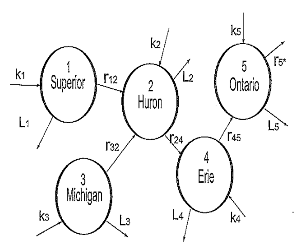
Along the border between the Middle and Eastern portions of the U.S. and Canda, there are five lakes called the Great Lakes. Consider the flow of a pollutant (such as PCB) into, out of, and between the Great Lakes and how one would model the concentration of pollution at time \(t\) (see figure below).
We begin by letting \(S(t),H(t), M(t),E(t)\) and \(O(t)\) represent the respective pollution concentrations (grams/liter) at time \(t\) (years) in lake Superior (1), Huron (2),Michigan (3), Erie (4) and Ontario (5). Next we define the following rate parameters:
\(r_{ij}\) is the transfer rate (year\(^{-1}\)) of pollution from lake \(i\) to lake \(j\) ;
\(k_i\) is the production rate of pollution (grams per liter per year) directly into lake \(i\); and
\(L_i\) is the rate of pollution purification treatment (year\(^{-1}\)) in lake \(i\).
We make the simplifying assumptions that within each lake (compartment) the pollution concentration is always uniform and the parameters \(r_{ij}\), \(k_i\) and \(L_i\) are all constant. Under such assumptions, a simple linear system of ODE’s can be used to describe the change in pollution concentrations in each lake (compartments):
Consider, for example, the rate of change at time \(t\) of pollution concentration in Huron \(\stackrel{.}{H}(t)\) (in grams/liter per year). This rate of change is equal to: RateIn - RateOut.
RateIn pollution enters in directly at the rate \(k_2\) (g/L per year) and also enters in from Superior at rate \(r_{12} S(t)\) (g/L per year) and from Michigan at rate \(r_{32}M(t)\) (g/L per year);
RateOut pollution leaves Huron to Erie at a rate \(r_{24} H(t)\) (g/L per year) and also leaves by purification treatment at rate \(L_2 H(t)\) (g/L per year).
The transfer of pollution between lakes is one-directional as determined by the flow of water.
Standard analysis of this type of model would include:
EQUILIBRIUM ANALYSIS We determine the equilibrium point (s,h,m,e,o) which gives the steady-state concentration levels in each lake by setting each differential equation equal to zero:
Observing that the functions \(F_i\) are differentiable with respect to \(S, H, M, E, O\) at the equilibrium point, we utilize the Jacobian matrix \(J\) which is computed as follows:
The eigenvalues of \(J\) determine the stability of the equilibrium point \((s,h,m,e,o)\). In particular, if all the eigenvalues are negative, the equilibrium is stable. In this case, as \(t\rightarrow\infty\) all solutions approach their equilibrium values; that is, \(S(t)\rightarrow s\), \(H(t)\rightarrow h\) \(M(t)\rightarrow m\), \(E(t)\rightarrow e\) and \(O(t)\rightarrow o\).
NUMERICAL ANALYSIS Assuming the rate constants can be estimated by direct measurements or other available data (see for example [Schnoor 1996]), we can use a differential equation solver to obtain the desired pollution concentration levels. If the equilibrium is stable, the equilibrium levels should appear in graphs of their respective pollution concentrations over sufficiently long time intervals.
SENSITIVITY ANALYSIS By varying of one or more of the rate parameters, we can assess the effectiveness of methods to reduce the amount of pollution in a particular lake or the total pollution concentration in all the lakes. For example, since \(s=\frac{k_1}{L_1+r_{12}}\), one can lower the equilibrium concentration in Superior by reducing \(k_1\) (regulating direct contamination), by increasing \(L_1\) (improving purification treatment), and/or by increasing \(r_{12}\) (increasing the outflow into Huron).
12.5.3. The CWS Model#
Now we will examine the CWS model in relation to Alzheimer’s. Craft, Wein and Selkoe [2002] created a model for the amyloid-beta biomarker concentrations in the brain, cerebral spinal fluid (“CSF”), and plasma. Clinically, changes in the concentrations of A\(\beta\) in the plasma and CSF are much easier to measure than in the brain. Changes in the CSF and plasma may then be useful to estimate the change in \(A\beta\) concentration level in the brain. The CWS model helps to determine the relationship between changes in these three compartments under different treatment scenarios.
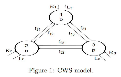
The CWS model can be viewed using compartments similar to the Great Lakes model, as shown in Figure 1. This model is based on several simplifying assumptions:
A\(\beta\) can exist as a single molecule (monomer) or as a chain of molecules (i.e. as a polymer) which connects \(i\) monomers (\(i=2,3,...\))
A\(\beta\) monomers exist in one of three disjoint compartments: the brain (1), cerebral-spinal fluid or CSF (2) and plasma (3)
A\(\beta\) polymers of any length can exist in the brain (polymer concentrations are assumed to be negligible outside the brain). Note: In Figure 1 compartment 4 is used to represent the polymers. This ``meta compartment” actually represents an infinite number of compartments, one for each polymer of length \(i\), (\(i=2,3,...\))
Each compartment has a homogeneous concentration of A\(\beta\)
In compartments 1, 2, and 3, A\(\beta\) monomers can be created or degraded (lost)
Monomers can be elongated by adjoining themselves to another monomer or to a polymer of any length
A polymer of length \(i\) can be elongated to a polymer of length \(i+1\)
A polymer of length \(i\) can be fragmented into a monomer and a polymer of length \(i-1\). (For more about polymer dynamics, see [Edelstein-Keshet, 2006]).
Under these assumptions, we let \(b_1(t)\) denote the A\(\beta\) monomer concentration in the brain, \(c(t)\) denote the A\(\beta\) monomer concentration in the CSF, \(p(t)\) denote the A\(\beta\) monomer concentration in the plasma, and \(b_i(t)\) represent the concentration of length \(i\) A\(\beta\) polymers in the brain. The following system of ordinary differential equations models the rate of change of the A\(\beta\) concentrations in each of the compartments:
(1)
(2)
(3)
(4)
Craft, Wein and Selkoe [2002] describe their model in the following way:
In Equation (1), the A\(\beta\) monomers in the brain are produced by cleavage of the Amyloid precursor protein (APP) at a constant rate of \(k_1\). The monomers live for \(L_1^{-1}\) time units before being lost. The same kind of production and loss occur in equations (3) and (4).
In Equations (1) and (2) we assume that the elongation occurs only by a monomer addition to a polymer with a rate constant \(E\). That is, \(E b_1(t)b_{i-1}(t)\) is the rate \((i-1)\)-mers elongate to \(i\)-mers.
Fragmentation occurs when a monomer breaks off at a rate \(F\) (i.e., \(i\)-mers fragment into an \((i-1)\)-mer and a monomer at rate \(F b_i(t)\)).
The factor of 2 in front of \(b_1(t)\) in equation (1) arises because it takes two monomers to form a dimer (polymer with length \(i\)=2).
The indicator variable \(I_{i=2}\) equals 1 if \(i=2\) and equals 0 otherwise; the factor \(\frac{1}{2}\) in front of \(I_i=2\) is due to the fact that a dimer can only fragment in one location, whereas longer \(i\)-mers have two possible fragmentation sites.
Equilibrium Analysis#
The CWS model is an infinite system of ODEs since it describes changes in the concentrations of polymers of length \(i=2,3,...\). Finding the equilibrium solutions of an infinite system is non-trivial, however it “leads to messy solutions and no insight into the problem” [Craft et. al. 2002, p.6]. So, Craft, Wein and Selkoe omit the straightforward approach and present a more intuitive method of finding the equilibrium solutions based on queueing networks [Jackson, 1957]. This more intuitive method is shown below:
These levels are determined by setting each of the differential equations equal to zero in the CWS model (Equations (1)-(4)):
(1’)
(2’) when \(i=2\)
(3’)
(4’)
These equations can be solved as follows:
Step 1: Use equations (3’) and (4’) to solve for \(c\) and \(p\) in terms of \(b_1\) and constants \(r_{ij},k_2,k_3,L_2,\) and \(L_3\).
In matrix form, equations (3’) and (4’) become:
(5)
where \(h_2=r_{21}+r_{23}+L_2\) and \(h_3=r_{31}+r_{32}+L_3\).
Letting \(\Delta=h_2 h_3 - r_{23}r_{32}\), the solution to (5) is
Step 2: Use equation (2’) to express \(b_2,b_3,b_4,...\) in terms of \(b_1\).
Adding the equations when \(i=1\), \(i=2\), \(i=3\), and \(i=4\) together leaves only \(Eb_1^2-\frac{1}{2}Fb_2=0\), or \(b_2=2b_1r\) where \(r=b_1\frac{E}{F}\).
Substituting this expression for \(b_2\) into equation (2’), we obtain \(b_3=2b_1r^2\). In a similar way, we can show \(b_i=2b_1r^{i-1}\), for \(i=2,3,...\).
Hence, once we find \(b_1\), we can compute \(b_2,b_3,...\), \(c\) and \(p\).
Step 3: Substitute \(b_i=2b_1r^{i-1}\) into equation (1’) to obtain \(b_1\).
This approach indicates:
The ratio \(r= b_1\frac{E}{F}\) is called the polymerization ratio. This a key parameter since all the polymer concentrations can be expressed in terms of \(r\) (in particular, \(b_i=2b_1r^{i-1}\)) and further, the total number of polymers forms a geometric series which is convergent if \(0\le r<1\) and divergent if \(r\ge 1\);
The steady state monomer concentration \(b_1\) is independent of the polymerization ratio \(r\); and
The total number of polymers \(b=\sum_{i=2}^{\infty} b_i= 2b_1 \sum_{i=2}^{\infty}r^{i-1} = b_1 \frac{2r}{1-r}\) (\(r<1\)) varies directly with \(b_1\).
Parameter Estimation#
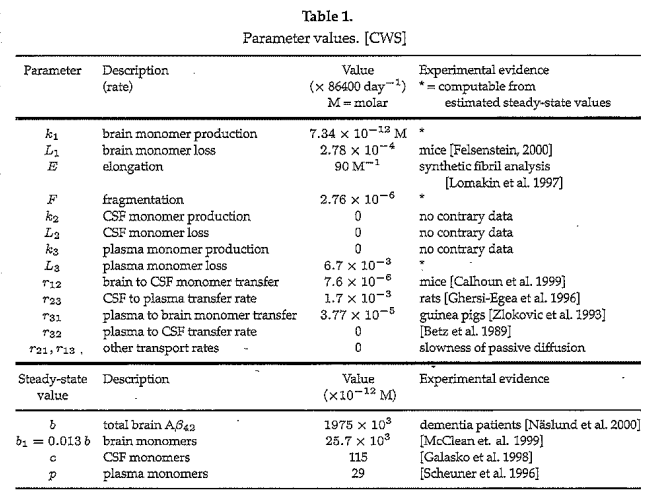
Assignment of specific values for the rate constants in a model is important and often challenging since real world phenomena are much more complex than their mathematical models. Moreover, in the case of AD, serious ethical issues and physical restrictions limit the type of experimental data which can be obtained. Table 1 gives the values used in the CWS model (with units standardized) and the source of these parameter values:
The 4 parameter values “computable from estimated steady state values,” obtained from experimental evidence, is particularly interesting. Craft, Wein and Selkoe provide an elegant approach to obtaining equilibrium values and their relationships to these 4 parameters as outlined in Table 2:
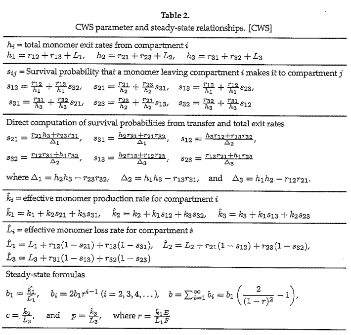
We explain the equations in Table 2 for compartment \(i=1\), the others being similar:
The total exit rate of monomers from the brain (\(h_1 = r_{12} + r_{13} + L_1\)) is the sum of the respective rates monomers move from brain to CSF (\(r_{12}\) ) and from brain to plasma (\(r_{13}\)), these being added to the loss of monomers in the brain by degradation (\(L_1\));
The survival probability that a monomer exiting the brain reaches the CSF (\(s_{12} = \frac{r_{12}}{h_1} + \frac{r_{13}}{h_1} s_{32}\)) is the probability that an exiting brain monomer goes directly to the CSF (\(\frac{r_{12}}{h_1}\)) plus the probability that a monomer first goes from brain to plasma and then transfers from plasma to CSF (\(\frac{r_{13}}{h_1}s_{32}\));
The effective production of monomers in the brain (\(\hat{k}_1 = k_1 + k_{2} s_{21} + k_{3} s_{31}\)) is the sum of direct production (\(k_1\)) plus the rate monomers transfer in from the CSF (\(k_{2} s_{21} \)) and from the plasma (\(k_{3} s_{31} \)); and
The effective loss of monomers in the brain (\(\hat{L}_1 = L_1 + r_{12}(1-s_{21}) + r_{13}(1-s_{31})\)) is due to degradation \(L_1\) and also by transfer out to and non-return from the CSF (\(r_{12}(1-s_{21})\)) and by transfer out to and non-return from the plasma (\(r_{13}(1-s_{31})\)).
12.5.4. A Simplified CWS Model#
The full CWS model (Equations (1)-(4)) does not have an exact solution nor can it be numerically integrated even with assigned parameter values because it is nonlinear and infinite dimensional. Therefore, the infinite system must be simplified in some way to a finite system. One such simplification is to approximate the CWS model monomer dynamics by removing the polymer compartment from the CWS model. In other words, we assume for simplicity that the values of \(E\) and \(F\) are negligible and set them both equal to zero. We keep all the other parameter values in Table 1 the same. The simplified CWS model based on only monomers being transferred takes the form of an autonomous linear system:
(L1)
(L2)
(L3)
Approximating the monomer dynamics may be useful as a measure of the total amyloid-beta concentration since, as we observed at the end of the last section, the total steady state polymer concentration varies directly with steady state monomer concentration \(b_1\). (Recall that an elevated total \(A\beta\) concentration level in the brain is thought to produce senile plaques which may be a major factor contributing to the progression of AD. (See [Luca et. al. 2003] for mathematical modeling related to plaque formation).
Since we use the same parameter values given in Table 1 for the simplified (linear) CWS model, the respective equilibrium values for monomers in the brain (\(b_1\sim 25,700\) pM), CSF (\(c\sim 115\) pM) and plasma (\(p\sim 29\) pM) remain the same as in Table 1. The stability of these equilibria is confirmed by computing the (constant) Jacobian matrix of the simplified model
and finding its eigenvalues, \(\{\)-582.136,-146.886,-24.652}, are all negative at the equilibrium point \((b_1,c,p)\).
Craft, Wein and Selkoe took a different approach to simplifying the infinite dimensional system by assuming that the total polymer concentration remains constant (\(\sum_{i=2}^{\infty} b_i(t)=S\) = constant). It is easy to show that their assumption leads to the following 3 dimensional non-linear system for \(b_1(t), c(t)\) and \(p(t)\):
(NL1)
(NL2)
(NL3)
where \(\tilde{k}_1=k_1 + F S\) and \(\tilde{L}_1=L_1 + E S\). Except for the non-linear term \(-2e b_1^2\) and adjusted parameter values \(\tilde{k}_1\) and \(\tilde{L}_1\) in (NL1), this system is identical to the linear system given by (L1).
We found that in all cases of interest these two simplified systems exhibited very similar numerical solution behavior (solutions are strongly attracted by the equilibrium values) and so will only graph numerical solutions to the simplified CWS model (L1) - (L3).
12.5.5. Analysis of Treatments#
Craft, Wein and Selkoe [2002] simulated a variety of treatment scenarios to assess the suitability of using \(A\beta\) monomer concentrations in the CSF and plasma to predict the \(A\beta\) monomer concentration in the brain. To illustrate and confirm their findings, we use the simplified CWS model (L1) - (L3) to simulate two of these treatment scenarios.
Treatment 1#
The first treatment scenario is to reduce the production of A\(\beta\) in the brain, that is, to lower the value of \(k_1\). For such a treatment, a \(\gamma\)-secretase inhibitor is used [Craft et. al. 2002]. (See [Das et. al. 2011] for further mathematical modelling on \(\gamma\)-secretase dynamics between the CSF and plasma). To simulate the effect of the treatment, we solve Equations L1- L3 numerically. We are assuming that a symptomatic patient is in a pre-treatment steady state on days 0-100 and is given a \(\gamma\)-secretase inhibitor that decreases the production rate \(k_1\) by 40% on days 100-465.
Show code cell source
import numpy as np
import matplotlib.pyplot as plt
from scipy.integrate import odeint

def f(y, t, params):
    b1, c,p = y      # unpack current values of y
    k1,k2,k3, r12,r13,r23,r21,r31,r32,L1,L2,L3 = params  # unpack parameters
    derivs = [k1*(1-.4*np.heaviside(t-100,0)+.4*np.heaviside(t-465,0))+r31*p+r21*c-(r13*b1+r12*b1)-L1*b1,      # list of dy/dt=f functions
             k2+r12*b1+r32*p-(r21*c+r23*c)-L2*c,
             k3+r13*b1+r23*c-(r31*p+r32*p)-L3*p,]
    return derivs

# Parameters
k1 = 7.34*86400
L1 = 24
k2=0
L2=0
k3=0
L3=6.7*10**(-3)*86400
r12=7.6*10**(-6)*86400
r23=1.7*10**(-3)*86400
r31=3.7*10**(-5)*86400
r32=0
r21=0
r13=0

# Initial values
b10 = 25.7*(10**3)
c0 = 115
p0 = 29

# Bundle parameters for ODE solver
params = [k1,k2,k3, r12,r13,r23,r21,r31,r32,L1,L2,L3 ]

# Bundle initial conditions for ODE solver
y0 = [b10,c0,p0]

# Make time array for solution
tStop = 1000.
tInc = 0.05
t = np.arange(0., tStop, tInc)

# Call the ODE solver
psoln = odeint(f, y0, t, args=(params,))

# Plot results
fig = plt.figure(1, figsize=(8,8))

# Plot b1 as a function of time
ax1 = fig.add_subplot(311)
ax1.plot(t, psoln[:,0])
ax1.set_xlabel('time')
ax1.set_ylabel('b1')

# Plot c as a function of time
ax2 = fig.add_subplot(312)
ax2.plot(t, psoln[:,1])
ax2.set_xlabel('time')
ax2.set_ylabel('c')

# Plot p as a function of time
ax3 = fig.add_subplot(313)
ax3.plot(t, psoln[:,2])
ax3.set_xlabel('time')
ax3.set_ylabel('p')
plt.savefig("treatment1.png")
plt.tight_layout()
plt.show()
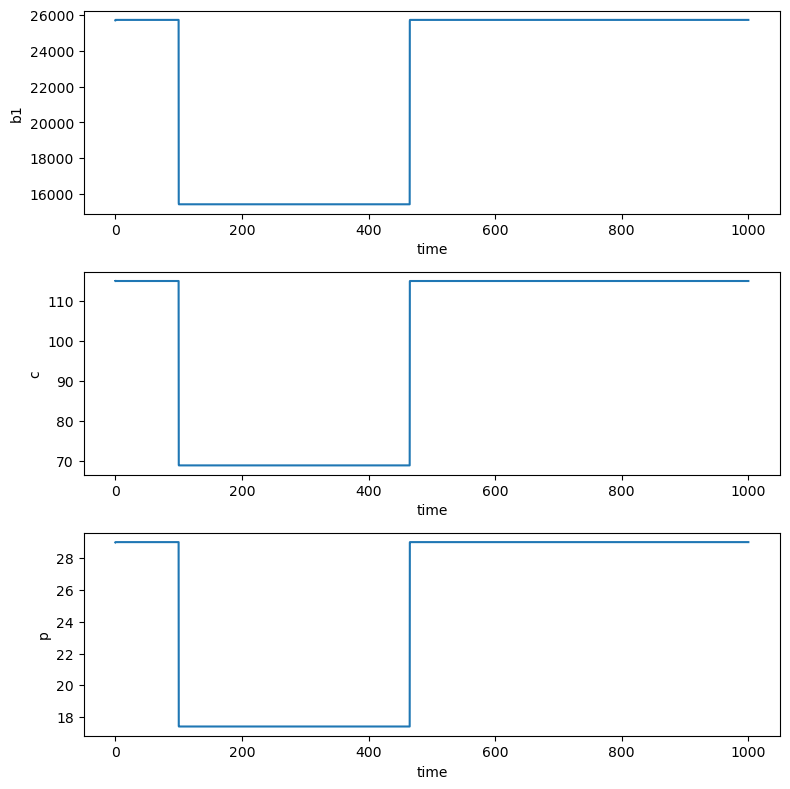
Treatment 1 results in the same Amyloid-beta level changes in the brain, CSF and plasma.
Treatment 2#
Our second treatment scenario is to change the transfer rate of A\(\beta\) between the brain and CSF. We will investigate what happens when \(r_{12}\) is increased by 100% on days 100-465. We simulate the effect of this treatment below. Why does this caution the use of Amyloid-beta as a biomarker for Alzheimer’s Disease?
Show code cell source
import numpy as np
import matplotlib.pyplot as plt
from scipy.integrate import odeint

def f(y, t, params):
    b1, c,p = y      # unpack current values of y
    k1,k2,k3, r12,r13,r23,r21,r31,r32,L1,L2,L3 = params  # unpack parameters
    derivs = [k1+r31*p+r21*c-(r13*b1+r12*b1*(1+np.heaviside(t-100,0)-np.heaviside(t-465,0)))-L1*b1,      # list of dy/dt=f functions
             k2+r12*b1*(1+np.heaviside(t-100,0)-np.heaviside(t-465,0))+r32*p-(r21*c+r23*c)-L2*c,
             k3+r13*b1+r23*c-(r31*p+r32*p)-L3*p,]
    return derivs

# Parameters
k1 = 7.34*86400
L1 = 24
k2=0
L2=0
k3=0
L3=6.7*10**(-3)*86400
r12=7.6*10**(-6)*86400
r23=1.7*10**(-3)*86400
r31=3.7*10**(-5)*86400
r32=0
r21=0
r13=0

# Initial values
b10 = 25.7*(10**3)
c0 = 115
p0 = 29

# Bundle parameters for ODE solver
params = [k1,k2,k3, r12,r13,r23,r21,r31,r32,L1,L2,L3 ]

# Bundle initial conditions for ODE solver
y0 = [b10,c0,p0]

# Make time array for solution
tStop = 1000.
tInc = 0.05
t = np.arange(0., tStop, tInc)

# Call the ODE solver
psoln = odeint(f, y0, t, args=(params,))

# Plot results
fig = plt.figure(1, figsize=(8,8))

# Plot b1 as a function of time
ax1 = fig.add_subplot(311)
ax1.plot(t, psoln[:,0])
ax1.set_xlabel('time')
ax1.set_ylabel('b1')

# Plot c as a function of time
ax2 = fig.add_subplot(312)
ax2.plot(t, psoln[:,1])
ax2.set_xlabel('time')
ax2.set_ylabel('c')

# Plot p as a function of time
ax3 = fig.add_subplot(313)
ax3.plot(t, psoln[:,2])
ax3.set_xlabel('time')
ax3.set_ylabel('p')
plt.savefig("treatment2.png")
plt.tight_layout()
plt.show()
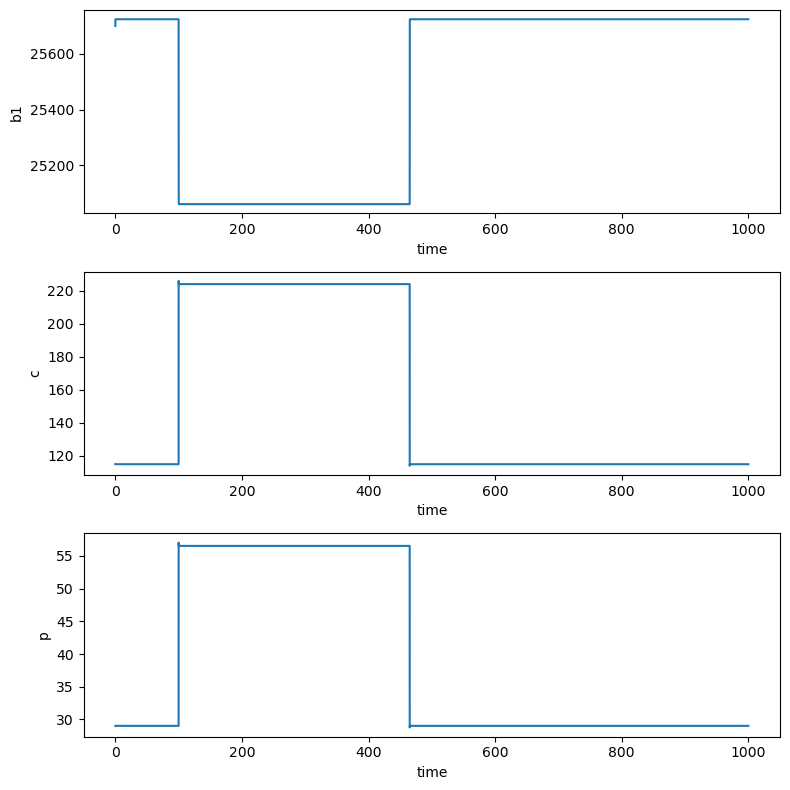
The A𝛽 concentration in the brain during treatment 2 decreases by 2.5% while the concentrations in the CSF and plasma both roughly double (in agreement with Figure 6 b-d in [Craft et. al. 2002]).
Note: Craft, Wein and Selkoe [2002] considered two other treatments:
A fragmentation enhancer increasing the fragmentation rate 100%; and
A vaccine which increases the monomer ingestion rate off of polymers by 100%.
In both these cases, the dynamics in all three compartments were similar.
12.5.6. Conclusion#
After simulating a variety of treatment scenarios, Craft, Wein and Selkoe concluded the need for caution about the use of A\(\beta\) as a biomarker. As exemplified by Treatment 1 and 2, relative changes in the A\(\beta\) levels are not uniform in all three compartments under all treatments. The effects of a particular treatment on the model parameters must be understood in order to correctly interpret clinical changes in a patient’s CSF and plasma A\(\beta\) levels.
Craft, Wein and Selkoe observe, for the case where the polymerization ratio satisfies \(r>1\), that though the values in Table 1 give \(r \sim .84\) and a total steady-state polymer concentration \(S\sim 1950\)x10\(^3\) pM, theoretically speaking, if \(r>1\), the steady state polymer concentration \(S\) becomes infinite. This implies that while the steady state brain monomer concentration \(b_1\) (which is independent of \(r\)) remains finite or is even reduced by some treatment, the total brain polymer concentration \(S=\sum_{i=2}^{\infty} b_i\) may increase without bound as each polymer concentration \(b_i\) approaches its finite steady state level (see Figure 5 in [Craft et. al. 2002]).
12.5.7. Exercises#
Exercises
The equilibrium analysis for Equation (2) of the CWS Model shown in this notebook is conducted for \(i=2\). Since \(i\) is the length of polymers, it is possible for \(i\) to equal 2, 3, 4, …. Using Equation (2) in the CWS Model, write what the equation used for equilibrium analysis of Equation (2) would be when \(i=3\) and \(i=4\).
Explain the equation for \(h_2\) in Table 2.
Why does the output for Treatment 2 caution the use of Amyloid beta as a biomarker for Alzheimer’s disease?
Simulate Treatment 2 using the non-linear model given by equations NL1-NL3. (Use the values \(E=S=0\) and \(F=.238\).) What do you observe?
12.5.8. References#
Calhoun, M., Burgermeister, P., Phinney, A., Stalder, M., Tolnay, M., Wiederhold, K.-H., Abramowski, D., Sturchler-Pierrat, C., Sommer, B., Staufenbiel, M. ad Jucker, M. 1999. Neurol overexpression of mutant amyloid pre-cursor protein results in prominent deposition of cerebrovascular amyloid. Neurobiology 96, 14088-14093.
Craft, D., Wein, L. and Selkoe,D. 2002. Mathematical model of the impact of novel treatments of the A\(\beta\) burden in the Alzheimer’s brain, CSF and plasma, Bulletin of Mathematical Biology, 64, 1011-1031.
Das, R. et. al. 2011. Modelling effect of a \(\gamma\)-Secratase inhibitor on amyloid-\(\beta\) dynamics reveals significant role of an amyloid clearance mechanism, Bulletin of Mathematical Biology, 73, 230-247.
Edekstein-Keshet, L. 2006. Simple models for polymer growth: implications for biopolymers, available at https://people.ok.ubc.ca/rtyson/Teaching/Math225/polymerize.pdf
Felsenstein, K. 2000. The next generation of AD therapeutics: the future is now. Abstracts from the 7th annual conference on Alzheimer’s Disease and Related Disorders, Abstract 613.
Galasko, D. et. al. 1998. High cerebrospinal fluid tau and low amyloid \(\beta42\) levels in the clinical diagnosis of Alzheimer disease and relation to Apolipoprotein E genotype, Archives of Neurology, 55, 937-945.
Ghersi-Egea, J.-F., Gorevic, P., Ghiso, J., Frangione, B., Patlak, C., Fenstermacher, J. 1996. Fate of cerebrospinal fluid-borne amyloid \(\beta\)-peptide: rapid clearance into blood and appreciable accumulation by cerebral arteries. Journal of Neurochemistry, 166, 880-883.
Jackson, J. 1957. “Networks of waiting lines” Operations Research, 5, pp. 518-521.
Johns H. and King L. 2011. “Larry King Interviews Harry Johns, President of the Alzheimer’s Association.” in the CNN special program Larry King Investigates Alzheimer’s. Available at https://web.archive.org/web/20140907054847/http://www.alzheimersreadingroom.com/2011/05/harry-johns-larry-king-investigates.html
Luca, M., Chavex-Ross, A, Edelestein-Keshet, L. and Mogilner A. 2003. Chemotactic signaling, microglia, and Alzheimer’s disease senile plaques: is there a connection?, Bulletin of Mathematical Biology,, 65, 693-730.*
McLean, C., Cherny, R., Fraser, F., Fuller, S., Smith, M., Beyreuther, K., Bush, A., Masters, C. 1999. Soluble pool of A\(\beta\) amyloid as a determinant of severity of neurodegeneration in Alzheimer’s Disease. Annals of Neurology, 46, 860-866.
N\(\ddot{a}\)slund, J., Haroutunian, V., Mohs, R., Davis, K., Davies, P., Greengard, P., Buxbaum, J. 2000. Correlation between elevated levels of amyloid \(\beta\)-peptide in the brain and cognitive decline. The Journal of the American Medical Association}, 283, 1571-1577.
Scheuner, D. et. al. 1996. Nature Medicine, 2, 864-870.
Schnoor, Jerald L. 1996. Environmental Modeling; Fate and Transport of Pollutants in Water, Air, and Soil, New York: John Wiley & Sons.
Thiess, W. 2010. Regarding ADNI Biomarkers Article from Archives of Neurology August 2010.
Zlokovic, B., Ghiso, J., Mackic, J., McComb, J., Weiss, M. and Frangione, B. 1993. Blood-brain barrier transport of circulating Alzheimer’s amyloid \(\beta\), Biochemical and Biophysical Research Communications, 197, 1034-1040.