13.5. Solutions to Exercises#
Section 2.1
2.1.1 1)\(\,\) a)\(\,\) \(1+8i\);\(\,\) b)\(\,\) \(3-2i\); \(\,\) c)\(\,\) \(-17+7i\);\(\,\) d)\(\,\) \(\frac{1}{2}-\frac{1}{2}i\); \(\,\) e)\(\,\) \(13-13i\)
2.1.2 \(\,\) a)\(\,\) \(e^{2x} \cos 2y+i(e^{2x} \sin 2y)\); \(\,\) b)\(\,\) \(\frac{1}{2}\, \ln((x+1)^2+y^2)+i\,\textrm{arctan}(\frac{ y}{x+1})\); \(\,\) c)\(\,\) \((x^2-y^2-1)+i\,(2xy)\)
2.1.3 If \(z_1=|z_1|e^{i\,\theta_1}\) and \(z_2=|z_2|e^{i\,\theta_2}\), then \(z_1 z_2=(|z_1|e^{i\,\theta_1})(|z_2|e^{i\,\theta_2})=|z_1| |z_2| e^{i(\theta_1+\theta_2)}\), from which we see \(|z_1 z_2|=|z_1| |z_2|\).
2.1.4 No, \(\arg(z_1z_2)=\arg(z_1)+ \arg(z_2)\)
Section 2.2
2.2.1 \(\lim_{h\rightarrow 0} \frac{10(z+h)^3-10z^3}{h}=\lim_{h\rightarrow 0} \frac{10z^3+30zh^2+30z^2h+10h^3 -10z^3}{h}=\lim_{h\rightarrow 0} \frac{30zh^2+30z^2h+10h^3}{h}=\lim_{h\rightarrow 0} 30zh+30z^2+10h^2=30z^2\)]
2.2.2
\(\lim_{h\rightarrow 0} \frac{\overline{z+h} - \bar{z} }{h}=\lim_{h\rightarrow 0} \frac{\bar{z}+\bar{h} - \bar{z} }{h}=\lim_{h\rightarrow 0} \frac{\bar{h} }{h}\)
Along the x-axis (h is real):
\(\lim_{h\rightarrow 0} \frac{\bar{h}} {h}=\lim_{h\rightarrow 0} \frac{h}{h}=1\). But, Along the y-axis (\(h=ik\), \(k\) real):
\(\lim_{k\rightarrow 0} \frac{\overline{ik}} {ik}=\lim_{k\rightarrow 0} \frac{-ik}{ik}=-1.\)
2.2.3 Using L’Hospital’s Rule, it follows that \(\lim_{z\rightarrow i} \frac{z^4-1}{z^8-1}= \lim_{z\rightarrow i} \frac{4z^3}{8z^7}=\lim_{z\rightarrow i} \frac{1}{2z^4} = \frac{1}{2}\).
Section 2.3
2.3.1 \(f(z)=[x+iy]^2= x^2-y^2 + i(2xy)\), so \(u(x,y)=x^2-y^2\) and \(v(x,y)=2xy.\) Thus \(u_x=2x = v_y\) and \(u_y=-2y=-v_x\) and the CR-eqns hold with the first partials all continuous functions. Moreover, we can use CR-eqns to obtain the derivative: \(f(z)= u_x+iv_x=2x+i2y=2z.\)
2.3.2 \(f(z)=x^2+y^2\), so \(u(x,y)=x^2+y^2\) and \(v(x,y)=0.\) Thus \(u_x=2x \neq v_y\) and the CR-eqns do not hold.
2.3.3 \(f(z)=e^{x+iy}=e^xe^{iy}=e^x\cos y + i e^x \sin y\). Thus, \(u=e^x \cos y\) and \(v=e^x \sin y\). Moreover, \(u_x=e^x\cos y = v_y\) and \(u_y=-e^x\sin y = -v_x\) so the C-R eqns hold with \(u_x,v_x,u_y,v_y\) all continuous, implying that \(f(z)\) is differentiable. Finally, \(f'(z)= u_x+iv_x= e^x\cos y + i e^x \sin y = e^z\) as expected.
2.3.4 Let \(f(z)=\log z = \ln r + i\theta\). Then \(u=\ln r\) and \(v=\theta\). Then \(u_r=\frac{1}{r} = \frac{1}{r} v_{\theta}\) and \(\frac{1}{r}u_{\theta}= 0 = -v_r\) so \(f(z)\) is differentiable (except when \(r=0\)). Moreover,
so the same formula for real calculus holds for the complex derivative of \(\log z\).
Section 2.4
2.4.1 a) Yes, \(\nabla^2 u_1=2-2=0\), so \(u_1\) is harmonic.; b) No, \(\nabla^2 u_2=2+2=4\neq 0\), so \(u_2\) is not harmonic; c) Yes, \(\nabla^2 u_3=0+0=0\), so \(u_3\) is harmonic.; d) Yes, \(\nabla^2 u_4=e^x\cos y-e^x\cos y=0\), so \(u_4\) is harmonic.; e) No, \(\nabla^2 u_5=-(\cos x + \cos y)\neq 0\), so \(u_5\) is not harmonic.
2.4.2 The harmonic conjugate of \(u_1\) is \(v_1= 2xy+C\), the harmonic conjugate of \(u_3\) is \(v_3=y+C\), and the harmonic conjugate of \(u_4\) is \(v_4=e^x\,\sin y+C\).
Section 2.5
2.5.1 First, \(\Psi=-y\). The family of lines can easily be visualized as the collection of vertical and horizontal lines in the plane, thus demonstrating that they are orthogonal.
2.5.2 a) \(u(x,y)=x^2-y^2\), \(v(x,y)=2xy\); b) Differentiating \(u(x,y)=\)constant and \(v(x,y)\)=constant with respect to \(x\), we obtain \(\frac{du}{dx}=\frac{x}{y}\) and \(\frac{dv}{dx}=-\frac{y}{x}\). Thus, the families of curves given by \(u(x,y)=c_1\) and \(v(x,y)=c_2\) have slopes that are opposite and reciprocal at any point of intersection, so the level curves are orthogonal.
Section 3
3.1 a) 0. There is no \(t\) dependence; b) \(2x\); c) 0. Satisfies continuity equation.
Section 3.2
3.2.1 \(\langle 4xe^{-y}, -2x^2e^{-y}\rangle\).
3.2.2 a) \(\nabla\cdot\) V =2y-2y=0. b) \(\Phi = \frac{y^3}{3} -x^2y \). c) \(\Phi_{xx}+\Phi_{yy}=2y-2y=0\)
Section 3.3
3.3.1 \(\Psi_y=\Phi_x=-\frac{q_u}{A}\Rightarrow \Psi= -\frac{q_u}{A} y + t(x)\)
\(t'(x)=\Psi_x=-\Phi_y=0 \Rightarrow t(x)=C\) and hence \(\Psi=-\frac{q_u}{A} y + C\)
\(\Omega = - \frac{q_u}{A}x -i\frac{q_u}{A} y +\Phi_0+ Ci =- \frac{q_u}{A} z +C_1.\) (Complex potential for uniform flow.)
The streamlines \(\Psi\)=constant are horizontal lines, and hence are perpendicular to the equipotentials \(\Phi\)=constant which are vertical lines.
Section 3.4
3.4.1 \(\Phi=x\) and \(\Psi=y\). The streamlines are horizontal (\(y\)=constant) and the flow is from right to left (higher to lower potential).
Section 3.5
3,5.1 The flow is from higher to lower velocity potential, hence from source to sink as expected.
Section 3.6
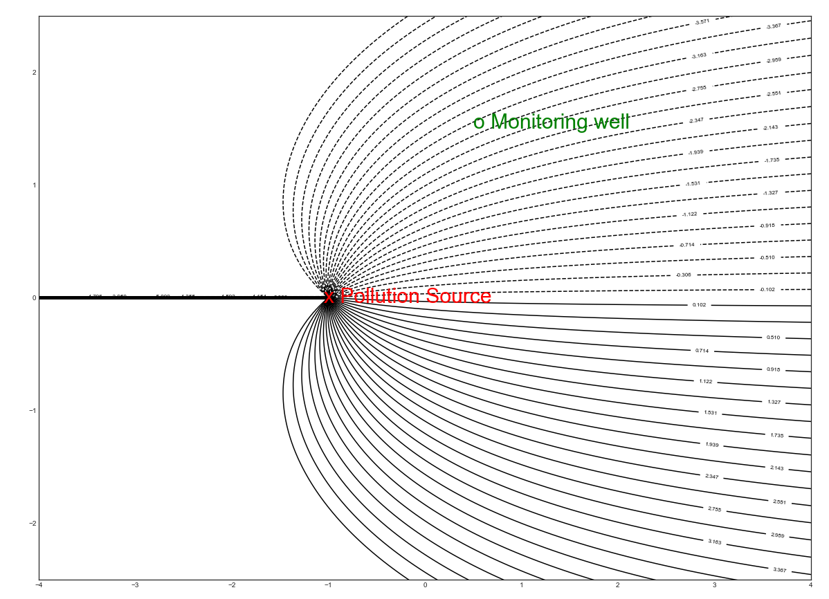
3.6.1 \(\Omega(z)=-z-2log(z+1)\) represents uniform flow with a source at \((-1,0)\) as shown in the Figure below.
3.6.2 a) \(\Psi(x,y)= -y-4\arctan\frac{Y-1}{X+8}+2\arctan\frac{Y-1}{X-1}-4\arctan\frac{Y+1}{X+8}+2\arctan\frac{Y+1}{x-1}\). b) 2 sinks and 2 sources c) The sources have twice the strength of the sinks. d) No. e) From the graph, there appears to be stagnation points at approximately (-13,0) and (3,0). f) \(\Omega'(z)=-1-\frac{4}{z-(-8+i)} +\frac{2}{z-(1+i)}-\frac{4}{z-(-8-i)}+\frac{2}{z-(1-i)}=0.\)
Section 4
4,1 See the JNB “Rotated Space-Leasing Plume” at wcapdat/GroundwaterFlow.
4.2 If we set \(k_1=3k\) and turn off EWSL-4 by setting \(k_2=0\), the complex potential becomes \(\Omega(z)=k_0z+3k\log(z)\). We then obtain the stagnation point from
For the stagnation to be located at \(z_{EWSL-4}=(10.8,0)\), we require that \(\hat{k}=\frac{-k_0(10.8)}{.3}\approx 5.22.\)
4.3 See the JNB “1NL Plume” at wcapdat/GroundwaterFlow.