import numpy as np
import matplotlib.pyplot as plt
import matplotlib.pyplot as plt
import numpy as np
from scipy.integrate import solve_ivp

12.2. Logistic Growth and COVID-19

12.2.1. Introduction

In this section, we explain the difference between exponential and logistic growth models using COVID-19 data reported by Wang et. al. in their 2020 paper “Prediction of epidemic trends in COVID-19 with logistic model and machine learning technics.”

12.2.2. Exponential Growth

Let \(y(t)\) represent the size of a specified population with \(y(0)=y_0\) the initial population size at time \(t=0\). The exponential growth model with positive, constant, growth rate \(k\)

\[ \frac{dy}{dt}=ky, \,\,\,\,y(0)=y_0 \]

is easily solved by separation of variables:

\[ \int \frac{dy}{y}=\,\int k\, dt \Rightarrow\ \ln y = kt + C \Rightarrow y = C_1 e^{kt}. \]

Using the intial condition \(y(0)=y_0\), we obtain

\[ y(t)=y_0e^{kt}. \]

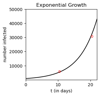
This model is able to predict rapid growth such as shown in the figure below:

Indeed, if we specify for example \(y(10)=5000\) and \(y(20)=30,000\), we have

\[ y(10)=y_0 e^{10k}=5000\Rightarrow y_0= 5000 e^{-10k} \]

\[ y(20)=y_0 e^{20k}=30,000\Rightarrow y_0 = 30000 e^{-20k}. \]

Setting these two expressions for \(y_0\) equal to each other gives

\[ 5000 e^{-10k}=30000e^{-20k}\Rightarrow e^{10k}=6 \Rightarrow 10k = \ln 6 \Rightarrow k=\frac{\ln(6)}{10}. \]

Using this value for \(k\), we can now find \(y_0\):

\[ y_0 = 5000 e^{-10k}\rightarrow y_0=5000 e^{-10\frac{\ln(6)}{10}}= 5000 e^{-\ln 6} = 5000 ( \frac{1}{6}) = 5000/6. \]

Let’s look at a graph of \(y=y_0e^{kt}\) for these values of \(k\) and \(y_0\).

Show code cell source Hide code cell source

k=np.log(6)/10
y0=5000/6

f = lambda t : y0 * np.exp(k*t)
t=np.arange(0,22,.01)
y=f(t)
plt.figure(figsize=(3,3))
plt.gca().set_xticks([0,10,20.])
plt.gca().set_yticks([10000,20000,30000,40000,50000])
plt.plot(t,y,'k',markersize=10)
plt.text(10,5000,'o',color='r')
plt.text(20,30000,'o',color='r')
plt.title('Exponential Growth')
plt.xlabel('t (in days)')
plt.ylabel('number infected')
plt.ylim((0,50000)) 
plt.xlim((0,22)) 
plt.show()

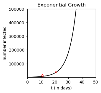
Any exponential growth function with \(y_0>0\) and \(k>0\) is such that \(\lim_{t\rightarrow\infty} y(t) =\infty\) , and thus is not realistic for predicting the spread of COVID-19 if the time horizon is sufficiently long. Observe in our case what happens if we extend, for example, the time horizon from \(t=0\) to \(t=50\).

Show code cell source Hide code cell source

f = lambda t : y0 * np.exp(k*t)
t=np.arange(0,50,.01)
y=f(t)
plt.figure(figsize=(3,3))
plt.gca().set_xticks([0,10,20,30,40,50])
plt.gca().set_yticks([100000,200000,300000,400000,500000])
plt.plot(t,y,'k',markersize=10)
plt.text(10,5000,'o',color='r')
plt.text(20,30000,'o',color='r')
plt.title('Exponential Growth')
plt.xlabel('t (in days)')
plt.ylabel('number infected')
plt.ylim((0,500000)) 
plt.xlim((0,50)) 
plt.show()

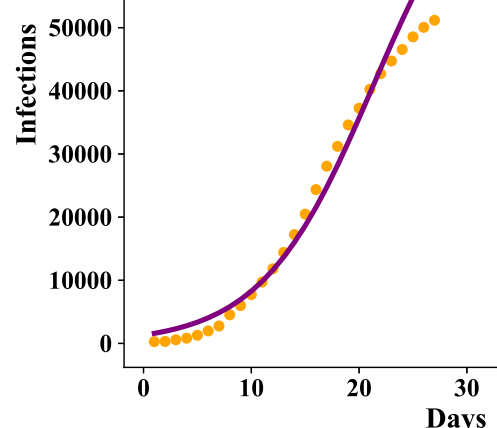
The actual reported data is shown below, and shows \(y(t)\) leveling off at about 80000.

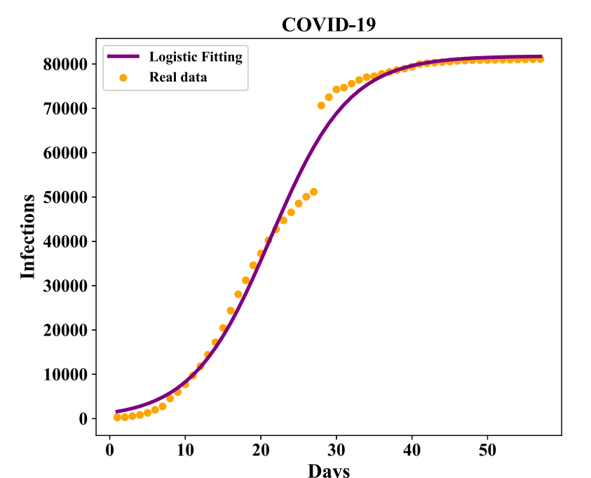
12.2.3. Logistic Growth Model

The logistic growth model

\[ \frac{dy}{dt}=ky(1-\frac{y}{M}), \,\,\,\,y(0)=y_0 \]

is used to describe “s-shaped” or “sigmoidal” growth. Note that when \(y\) is small compared to \(M\), then

\[ \frac{dy}{dt}\approx ky \]

so we he have exponential growth.

However, as \(y\) approaches \(M\), the factor \((1-\frac{y}{M})\) approaches 0, and so \(\frac{dy}{dt}\rightarrow 0\).This achieves the “leveling off” of the growth.

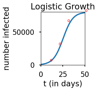
Let’s numerically solve the logistic growth model for the values \(k=\log(6)/10\), \(y_0=5000/6\) and \(M=80000\).

Show code cell source Hide code cell source

plt.style.use('seaborn-poster')

%matplotlib inline

k=np.log(6)/10
y0=5000/6
M=80000

F = lambda t,y: k*y*(1-y/M)

t_eval = np.arange(0, 50, 0.01)
sol = solve_ivp(F, [0, 50], [y0], t_eval=t_eval)

plt.figure(figsize = (3,3))
plt.plot(sol.t, sol.y[0])
plt.text(10,5000,'o',color='r')
plt.text(20,30000,'o',color='r')
plt.text(30,65000,'o',color='r')
plt.text(50,80000,'o',color='r')


plt.title('Logistic Growth')
plt.xlabel('t (in days)')
plt.ylabel('number infected')
plt.ylim((0,80000)) 
plt.xlim((0,50)) 
plt.tight_layout()
plt.show()

C:\Users\pisihara\AppData\Local\Temp\ipykernel_22672\137539061.py:1: MatplotlibDeprecationWarning: The seaborn styles shipped by Matplotlib are deprecated since 3.6, as they no longer correspond to the styles shipped by seaborn. However, they will remain available as 'seaborn-v0_8-<style>'. Alternatively, directly use the seaborn API instead.
  plt.style.use('seaborn-poster')

12.2.4. Exercises

Exercises

1. Use separation of variables and partial fractions to obtain the general solution to the logistic model

\[ \frac{dy}{dt}=ky(1-\frac{y}{M})\,\,\,y(0)=y_0 \]

2. a) Make a plot of the logistic model solutions for the values \(k=1\), \(M=100\) for \(y_0=10\), \(y_0=50\), \(y_0=90\), and \(y_0=110\).

b) Sketch a slope field to explain qualitatively the behavior of the general logistic model for \(k>0\) and \(M>0\). Sketch solution curves where a) \(y_0\) is close to 0; b) \(y_0\) is roughly \(M/2\); c) \(y_0\) is slightly smaller than \(M\); and d) \(y_0\) is slightly greater than \(M\)

Reference

Wang, P., Zheng, X., Li, J., and Zhu, B. 2020. Prediction of epidemic trends in COVID-19 with logistic model and machine learning technics. Chaos, Solitons, and Fractals, 139(2020), 1-7.