8.2. Functions#
Note
Below is the list of topics that are covered in this section:
Function Definition and Terminology
Function Behaviors
Common Functions (Linear, Exponential, Logarithm, Logistic)
Function Operations, Compositions, and Inverse
import sympy as sp
import numpy as np
import matplotlib.pyplot as plt
8.2.1. Function Definition and Terminology#
A function is a rule that assigns exactly one output to each input. When a function \(f\) has input \(x\), the output is written \(f(x)\). This notation is read “\(f\) of \(x\)”.
Example 1
\(f(x)=x+3\) is a rule that adding \(3\) into the input \(x\), giving the output \(x+3\).
\(g(x)=8-x^2\) is a rule that squaring the input \(x\), then subtracting the result from \(8\), giving the output \(8-x^2\).
Code example for \(f(x)=x+3\) is given below. Enter an input value and the code will return the output value.
Show code cell source
#define the function f(x)
def f(x):
    return x+3

# Ask for user input (uncomment the next line if using an interactive JNB)
user_input = float(input("Enter input value x ="))

# Call the function with the user input
output = f(user_input)

# Print the output
print("The output is f(x) =", output)
Enter input value x =1
The output is f(x) = 4.0
The domain of a function is the set of all input values that can be plugged into a function such that the output exists.
The range of a function is the set of all possible output values that a function can take.
Note that for the domain we need to avoid division by zero, square roots of negative numbers, and logarithms of nonpositive numbers. Can you explain why?
Python itself does not have built-in functionality to directly determine the domain and range of a given function. The domain and range of a function often depend on the specific characteristics of the function and its mathematical properties.
Example 2
Given \(f(x)=\frac{1}{\sqrt{x}}\).
Excluding the zeroes of the denominator and negative number inside the square root, the domain of \(f(x)\) is \(\left(0,\infty\right)\). The range of \(f(x)\) hence also \(\left(0,\infty\right)\).
Code example for \(f(x)\) is given below.
# Define the function symbolically
x = sp.Symbol('x')
f = 1 / (sp.sqrt(x))

# Find the domain: denominator not zero AND inside square root must be positive
domain = sp.solve(sp.denom(f) != 0 and x>0, x)

# Print the domain
print("Domain:", domain)
Domain: (0 < x) & (x < oo)
8.2.2. Function Behaviors#
Increasing, Decreasing, and Constant Function#
A function \(f\) defined over an interval is:
increasing if the output values increase as the input values increase.
decreasing if the output values decrease as the input values increase.
constant if the output values remain the same as the input values increase.
Concave Up and Concave Down Function, Inflection Point#
A function \(f\) defined over an interval is:
concave up if a graph of \(f\) appears to be a portion of an arc opening upward.
concave down if a graph of \(f\) appears to be a portion of an arc opening downward.
A point on a function changes concavity is called an inflection point.
8.2.3. Common Functions (Linear, Exponential, Logarithm, Logistic)#
Linear Functions#
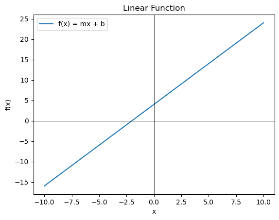
A linear function is a function that can be expressed in the form \(f(x)=mx+b\), where \(m\) represents the slope and \(b\) represents the \(y\)-intercept.
The slope \(m\):
Determines the steepness or inclination of the line. A positive slope indicates an upward trend, a negative slope indicates a downward trend, and a slope of zero represents a horizontal line.
Represents the rate at which the function’s output changes with respect to the input.
Is calculated as the ratio of the change in \(y\)-coordinates to the change in \(x\)-coordinates between two points on the line, that is, between point \((x_1,y_1)\) and \((x_2,y_2)\), the slope \(m=\dfrac{y_2-y_1}{x_2-x_1}\).
The \(y\)-intercept \(b\):
Is the point where the line intersects the \(y\)-axis.
Represents the value of the \(f(x)\) when \(x = 0\).
To find the \(x\)-intercept, set \(y = 0\) in the equation \(f(x)=mx+b\) and solve for \(x\).
Below is the code prompting user to input the constants \(m\), and \(b\).
Show code cell source
# Prompt the user to input the slope and y-intercept
m = float(input("Enter the value for the slope (m): "))
b = float(input("Enter the value for the y-intercept (b): "))

# Define the linear function
def linear_function(x):
    return m * x + b

# Generate a range of x values for plotting
x = np.linspace(-10, 10, 100)

# Compute the corresponding y values using the linear function
y = linear_function(x)

# Plot the linear function
plt.plot(x, y, label='f(x) = mx + b')

# Plot the x-axis and y-axis lines
plt.axhline(0, color='black', linewidth=0.5)  # x-axis
plt.axvline(0, color='black', linewidth=0.5)  # y-axis

# Set plot labels and title
plt.xlabel('x')
plt.ylabel('f(x)')
plt.title('Linear Function')

# Add a legend
plt.legend()

# Display the plot
plt.show()
Enter the value for the slope (m): 2
Enter the value for the y-intercept (b): 4
Exponential Functions#
An exponential function is a function in the form \(f(x)=ab^x\), where \(a\) is the \(y\)-intercept and \(b>0\) is the constant multiplier.
Below is the code to plot the graphs of \(f(x)=2^x\) and \(f(x)=\left(\frac{1}{2}\right)^x\):
Show code cell source
# Define the x range
x = np.linspace(-3, 3, 100)

# Define the functions
f1 = 2 ** x
f2 = (1 / 2) ** x

# Plot the functions
plt.plot(x, f1, label='f(x) = 2^x')
plt.plot(x, f2, label='f(x) = (1/2)^x')

# Plot the x-axis and y-axis lines
plt.axhline(0, color='black', linewidth=0.5)  # x-axis
plt.axvline(0, color='black', linewidth=0.5)  # y-axis

# Set plot labels and title
plt.xlabel('x')
plt.ylabel('f(x)')
plt.title('Plot of f(x) = 2^x and f(x) = (1/2)^x')

# Add a legend
plt.legend()

# Display the plot
plt.show()
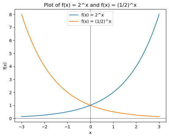
Properties of \(f(x)=ab^x\):
\(f(0)=a\). The \(y\)-intercept is always at \(y=a\).
\(f(x) > 0\). An exponential function is always positive (never touch zero either)
The domain of \(f(x)\) is \((-\infty,\infty)\) while the range of \(f(x)\) is \((0,\infty)\).
If \(0<b<1\) then
\(f(x)\) goes to \(0\) as \(x\) goes to \(\infty\).
\(f(x)\) goes to \(\infty\) as \(x\) goes to \(-\infty\).
If \(b>1\) then
\(f(x)\) goes to \(\infty\) as \(x\) goes to \(\infty\).
\(f(x)\) goes to \(0\) as \(x\) goes to \(-\infty\).
The natural exponential function is \(f(x)=e^x\), where \(e\) is the Euler’s number \(e=2.71828182845905\ldots\)
Logarithm Functions#
A logarithm (log) function is a function in the form \(f(x)=a+b\ln(x)\), where \(a\) and \(b\neq 0\) are constants for positive input \(x\).
Below is the code to plot the graphs of \(f(x)=1+2\ln(x)\) and \(f(x)=1-2\ln(x)\):
Show code cell source
# Define the functions
def f1(x):
    return 1 + 2 * np.log(x)

def f2(x):
    return 1 - 2 * np.log(x)

# Generate a range of x values for plotting
x = np.linspace(0.1, 10, 100)

# Compute the corresponding y values for each function
y1 = f1(x)
y2 = f2(x)

# Plot the functions
plt.plot(x, y1, label='f(x) = 1 + 2 * ln(x)')
plt.plot(x, y2, label='f(x) = 1 - 2 * ln(x)')

# Plot the x-axis and y-axis lines
plt.axhline(0, color='black', linewidth=0.5)  # x-axis
plt.axvline(0, color='black', linewidth=0.5)  # y-axis

# Set plot labels and title
plt.xlabel('x')
plt.ylabel('f(x)')
plt.title('Plot of f(x) = 1 + 2 * ln(x) and f(x) = 1 - 2 * ln(x)')

# Add a legend
plt.legend()

# Display the plot
plt.show()
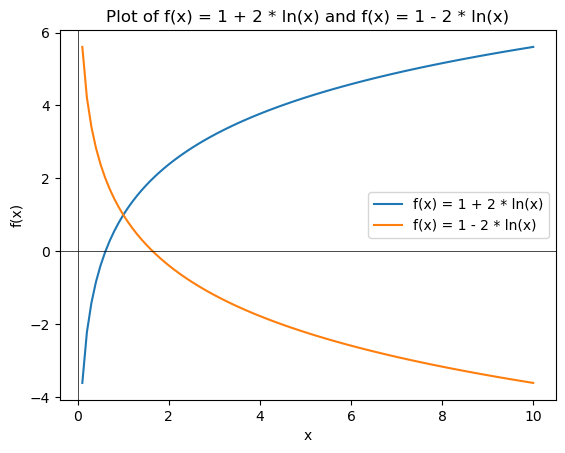
Properties of \(f(x)=a+b\ln(x)\):
The input \(x\) is restricted to be positive since \(\ln(x)\) is only defined for \(x>0\).
The log function then can be either increasing or decreasing depending on the value of \(b\).
For increasing log functions:
concave down
\(b>0\)
vertical asymptote \(x=0\), with \(f(x)\) goes to \(-\infty\)
\(f(x)\) goes to \(\infty\) as \(x\) goes to \(\infty\)
For decreasing log functions:
concave up
\(b<0\)
vertical asymptote \(x=0\), with \(f(x)\) goes to \(\infty\)
\(f(x)\) goes to \(-\infty\) as \(x\) goes to \(\infty\)
Logistic Functions#
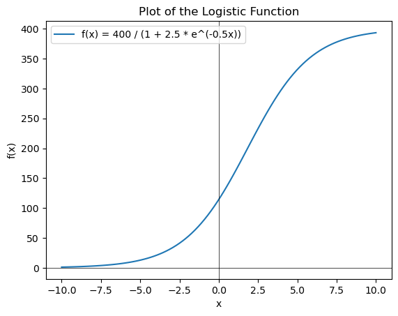
While exponential and log functions are commonly used in real life, it is unrealistic to believe that exponential growth can continue forever. In many situations, the growth ultimately restricted by the logistic availability.
A logistic function is a function in the form \(f(x)=\dfrac{L}{1+ae^{-bx}}\), where \(L,a\), and \(b\) are nonzero constant.
In this function, \(y=0\) and \(y=L\) are the horizontal asymptotes of the graph of \(f(x)\), corresponding to the fact that the amount of resources is always positive but the growth is limited at a certain point.
Depending on the positive or negative growth of the logistics, the logistic function can either increase or decrease.
Below is an example of the graph of an increasing logistic function \(f(x)=\dfrac{400}{1+2.5e^{-0.5x}}\):
Show code cell source
# Define the x range
x = np.linspace(-10, 10, 100)

# Define the logistic function
f = 400 / (1 + 2.5 * np.exp(-0.5 * x))

# Plot the logistic function
plt.plot(x, f, label='f(x) = 400 / (1 + 2.5 * e^(-0.5x))')

# Plot the x-axis and y-axis lines
plt.axhline(0, color='black', linewidth=0.5)  # x-axis
plt.axvline(0, color='black', linewidth=0.5)  # y-axis

# Set plot labels and title
plt.xlabel('x')
plt.ylabel('f(x)')
plt.title('Plot of the Logistic Function')

# Add a legend
plt.legend()

# Display the plot
plt.show()
Below is the code prompting user to input the constants \(L, a\), and \(b\).
Show code cell source
# Prompt the user to input the parameters
L = float(input("Enter the value for L: "))
a = float(input("Enter the value for a: "))
b = float(input("Enter the value for b: "))

# Define the logistic function
def logistic_function(x):
    return L / (1 + a * np.exp(-b * x))

# Generate a range of x values for plotting
x = np.linspace(-10, 10, 100)

# Compute the corresponding y values using the logistic function
y = logistic_function(x)

# Plot the logistic function
plt.plot(x, y, label='f(x) = L / (1 + a * e^(-b * x))')

# Plot the x-axis and y-axis lines
plt.axhline(0, color='black', linewidth=0.5)  # x-axis
plt.axvline(0, color='black', linewidth=0.5)  # y-axis

# Set plot labels and title
plt.xlabel('x')
plt.ylabel('f(x)')
plt.title('Logistic Function')

# Add a legend
plt.legend()

# Display the plot
plt.show()
Enter the value for L: 10
Enter the value for a: 1
Enter the value for b: 2
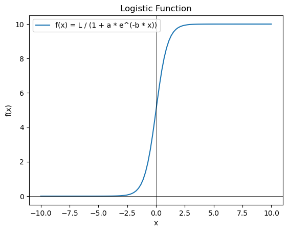
Properties of \(f(x)=\dfrac{L}{1+ae^{-bx}}\):
For increasing logistic function:
The function begins concave up then changes to concave down
\(b>0\)
Horizontal asymptotes \(y=0\) to the left and \(y=L\) to the right
For decreasing logistic function:
The function begins concave down then changes to concave up
\(b<0\)
Horizontal asymptotes \(y=L\) to the left and \(y=0\) to the right
Both increasing and decreasing logistic functions have exactly one inflection point.
Without further contextual restriction on the domain, the domain of a logistic function is \((-\infty,\infty)\) and the range is \((0,L)\).
8.2.4. Function Operations, Compositions, and Inverse#
Function Operations#
Note that not everything can be mathematically operated. To show a simple example, adding apples and oranges does not equal an exclusive number of either apples or oranges. If given context, it is important to pay attention to what you are trying to operate. As mentioned in the Introduction section, we focus on the values rather than the contexts in this Calculus module.
If the input \(x\) of functions \(f\) and \(g\) are well-defined for the functions to be operated, then the following new functions can be constructed:
function addition: \([f+g](x)=f(x)+g(x)\)
function subtraction: \([f-g](x)=f(x)-g(x)\)
function multiplication: \([f\cdot g](x)=f(x) \cdot g(x)\)
function division: \(\left[\dfrac{f}{g}\right](x)=\dfrac{f(x)}{g(x)}\), where \(g(x)\neq 0\)
Example 3
Below is a code example that prompts the user to input a value of \(x\), as well as two functions \(f(x)\) and \(g(x)\).
It then computes and returns the sum, difference, product, and quotient of the functions at the given value of \(x\).
Note that \(g(x)\) cannot be zero at the given input \(x\).
Show code cell source
def calculate_operations(f, g, x):
    # Evaluate f(x) and g(x)
    f_value = f(x)
    g_value = g(x)

    # Compute sum, difference, product, and quotient
    sum_result = f_value + g_value
    difference_result = f_value - g_value
    product_result = f_value * g_value
    quotient_result = f_value / g_value

    # Return the results
    return sum_result, difference_result, product_result, quotient_result

# Prompt the user to enter the value of x
x = float(input("Enter the value of x: "))

# Prompt the user to enter the functions as strings
f_input = input("Enter the first function (f(x)): ")
g_input = input("Enter the second function (g(x)): ")

# Create the functions from the user input
f = eval("lambda x: " + f_input)
g = eval("lambda x: " + g_input)

# Calculate the operations at the given value of x
sum_result, difference_result, product_result, quotient_result = calculate_operations(f, g, x)

# Print the results
print("Sum:", sum_result)
print("Difference:", difference_result)
print("Product:", product_result)
print("Quotient:", quotient_result)
Enter the value of x: 3
Enter the first function (f(x)): x**2
Enter the second function (g(x)): 3*x-1
Sum: 17.0
Difference: 1.0
Product: 72.0
Quotient: 1.125
Function Compositions#
The function composition of two functions is evaluated by plugging one function into the other function. The composition operator is \(\circ\).
\((f\circ g)(x)=f(g(x))\)
\((g\circ f)(x)=g(f(x))\)
Example 4
Given \(f(x)=3x^2+10\) and \(g(x)=1-2x\).
\((f\circ g)(x)=f(g(x))=f(1-2x)=3(1-2x)^2+10\)
\((g\circ f)(x)=g(f(x))=g\left(3x^2+10\right)=1-2\left(3x^2+10\right)\)
\((g\circ g)(x)=g(g(x))=g(1-2x)=1-2\left(1-2x\right)\)
To create a composition function of two user functions at a certain input value, you can prompt the user to enter the functions as strings and dynamically evaluate and compose them.
For \((f\circ g)(x)\) from above example:
Show code cell source
def compose_functions(f, g):
    def composed_function(x):
        return f(g(x))
    return composed_function

# Prompt the user to enter the functions as strings
f_input = input("Enter the first function: ")
g_input = input("Enter the second function: ")

# Create the functions from the user input
f = eval("lambda x: " + f_input)
g = eval("lambda x: " + g_input)

# Create the composition function
composed = compose_functions(f, g)

# Prompt the user to enter an input value
x = float(input("Enter the input value: "))

# Compute the composition of the user input functions
result = composed(x)
print("Result:", result)
Enter the first function: x**2
Enter the second function: 3*x+1
Enter the input value: 3
Result: 100.0
Inverse Functions#
Given a one-to-one function, a new function can sometimes be created by reversing the input and output of the original function. This reversed function is called an inverse function.
The inverse function of a one-to-one function \(f(x)\) is denoted \(f^{-1}(x)\).
Composing a function and its inverse will undo what each of the functions do to the input \(x\), hence \(\left(f\circ f^{-1}\right)(x)=x\) and \(\left(f^{-1}\circ f\right)(x)=x\).
Example 5
Given \(f(x)=2x+3\). What \(f\) does here is first multiply \(x\) by \(2\), then adding the result by \(3\).
To reverse what \(f\) does, we took the reverse of the action backward. The reverse of “add \(3\)” is “subtract \(3\)”. Reverse of “multiply by \(2\)” is “divide by \(2\)”.
This means the inverse function first subtracts the input \(x\) by \(3\), then divides the result by \(2\). Hence the inverse function is \(f^{-1}(x)=\frac{x-3}{2}\).
This can easily checked by confirming that \(\left(f\circ f^{-1}\right)(x)=x\) and \(\left(f^{-1}\circ f\right)(x)=x\).
Below is a code example that prompts the user to input a function \(f(x)\) and \(x=a\), and then calculates and returns \(f^{-1}(a)\). Note that the user must input a one-to-one function.
Show code cell source
def find_inverse(f):
    def inverse(x):
        # Use a binary search algorithm to find the inverse
        left = -1000  # Starting point for search
        right = 1000  # Ending point for search
        precision = 0.0001  # Precision of the inverse calculation

        while right - left > precision:
            mid = (left + right) / 2
            if f(mid) < x:
                left = mid
            else:
                right = mid

        return round((left + right) / 2, 4)  # Return the approximate inverse with 4 decimal places

    return inverse

# Prompt the user to enter the function f(x) as a string
f_input = input("Enter the function f(x): ")

# Create the function from the user input
f = eval("lambda x: " + f_input)

# Calculate the inverse function
inverse_f = find_inverse(f)

# Prompt the user to enter a value for x
x = float(input("Enter a value for x: "))

# Calculate the inverse of f(x) at the given x value
inverse_result = inverse_f(x)

# Print the result
print("Inverse of f(x) at x =", x, "is approximately:", inverse_result)
Enter the function f(x): x**3
Enter a value for x: 4
Inverse of f(x) at x = 4.0 is approximately: 1.5874
8.2.5. Exercises#
Exercises
Find the domain of the following functions.
\(f(x)=\sqrt{x-9}\)
\(f(x)=\dfrac{1}{\sqrt{x}-9}\)
\(f(x)=\ln(x-9)\)
Given the graph of the function \(f\) below.
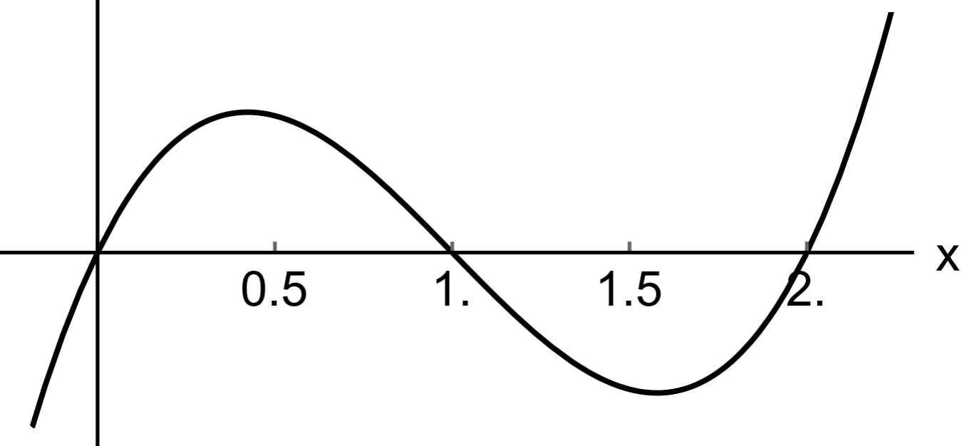
Find the intervals on which the graph of \(f\) is increasing or decreasing
Find the intervals on which the graph of \(f\) is concave up or concave down
Find the inflection points (if any)
Plot the following functions on the interval \([-5,5]\):
\(f(x)=4+3x\)
\(f(x)=4\cdot 3^x\)
\(f(x)=4+3\log(x)\)
\(f(x)=4\cos(3x)\)
\(f(x)=\dfrac{1.5}{1+4e^{-2.45x}}\)
Given \(f(x)=1+6x^2\) and \(g(x)=6-\sqrt{x}\). Find each of the following:
\([f+g](1234)\)
\((g\circ f)(2345)\)
\([f\cdot g](0.3456)\)
\((f\circ f)(4567)\)
\(g^{-1}(0.2345)\)