Show code cell source
import matplotlib.pyplot as plt
import numpy as np
7.16. JNB Lab Solutions#
Exercise 1.1
a)
Show code cell source
plt.figure(figsize=(8, 4))
plt.xlim=[0,1]
plt.ylim=[0,.1+np.log(.5)]
p=np.linspace(0.001,.999,1000)
H= -(p * np.log(p) + (1-p) *  np.log(1-p))
plt.plot(p,H,color='r')
plt.grid()
plt.xlabel("p")
plt.ylabel("H")
plt.show()
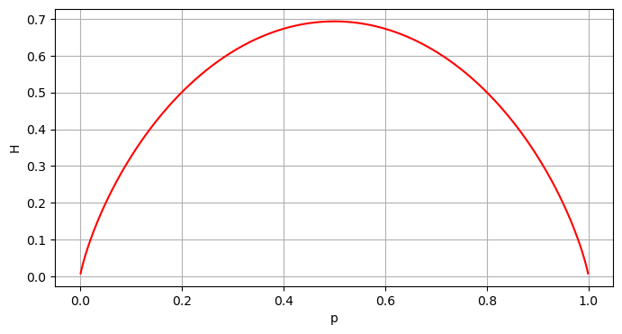
b) Note that \(H(p)=H(1-p)\), so \(\lim_{p\rightarrow 0^+}H(p)=\lim_{p\rightarrow 1^-}H(p)\).
Using L’Hospital’s Rule,
Furthermore, \(\lim_{p\rightarrow 0^+}-(1-p)\ln (1-p)=\lim_{q\rightarrow 1^-} -q \ln q = 0\). The desired result follows.
c)
Let \(H(p)= -[p\ln p + (1-p)\ln(1-p)]\). Then
Moreover, for values of \(p\) near \(p=.5\), if \(p<.5\) then \(H'(p)>0\) so \(H\) is increasing, and if \(p>.5\), then \(H'(p)<0\) so \(p\) is decreasing. This implies \(H(.5)\) is a max.
Note that in this case \(H''(.5)=0\) so the second derivative test does not apply.
Exercise 2.1
a), b), and c) all have the same value of H= -(.5 ln .5 + .3ln .3 + .2 ln .2) \(\approx\) 1.03.
Which option is labeled “1”, “2” or “3” is inconsequential in the computation of the entropy of disagreement. (Note that this makes it difficult to apply entropy to a histogram where the bin numbers are purposefully ordered. For example, the label i might mean a student fails i tests in a particular math course.)
Exercise 3.1
a) \(\int_0^{\infty} ke^{-kx}\,dx = -e^{-kx}\mid_0^{\infty}=0+1=1.\)
b) The mean \(E(X)\) is given by the integral \(E(X)=\int_0^{\infty} (kx) e^{-kx}\,dx.\) Using integration by parts with \(u=kx\), \(du=k\,dx\), \(dv=e^{-kx}\,dx\), \(v=-(1/k)e^{-kx}\), we have
\(E(X)= - xe^{-kx}\mid_{x=0}^{\infty} + \int_{x=0}^{\infty} -e^{-kx}\,dx= 0 -(1/k)e^{-kx}\mid_{x=0}^{\infty}=1/k.\)
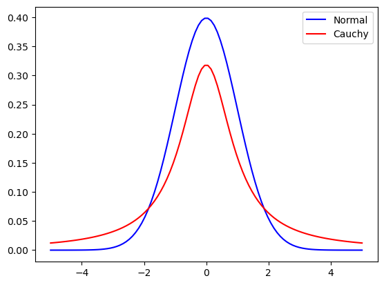
Exercise 4.1
a)
Show code cell source
import math
import random
import scipy.stats as stats
from scipy.stats import powerlaw
mu = 0
variance = 1
sigma = math.sqrt(variance)
x = np.linspace(mu - 5*sigma, mu + 5*sigma, 100)
plt.plot(x, stats.norm.pdf(x, mu, sigma),color='b')
plt.plot(x, stats.cauchy.pdf(x, mu, sigma),color='red')
plt.legend(["Normal","Cauchy"])
plt.show()
b)
Show code cell source
trials=10000
class_size=10
s = np.random.standard_cauchy(trials*class_size)

Hroutine=[]
Hexceptional=[]
Hsum=[]
k=0

for j in np.arange(0,trials,1):
    routine=0
    exceptional=0
    for i in np.arange(0,10,1):
        if s[k]>3 or s[k]<-3:
            exceptional=exceptional+1
            k=k+1
        else:
            routine=routine+1
            k=k+1
    if routine>0:
        p=routine/10
        Hroutine.append(-p*np.log(p))
    else:
        Hroutine.append(0)
    if exceptional>0:
        p=exceptional/10
        Hexceptional.append(-p*np.log(p))
    else:
        Hexceptional.append(0)
    Hsum.append(Hroutine[j]+Hexceptional[j])


H=np.mean(Hsum)
Hex=np.mean(Hexceptional)

print("Entropy of Cauchy Class=", H)
print("Contribution to Entropy by Exceptional Students=", Hex)
Entropy of Cauchy Class= 0.4498874005479002
Contribution to Entropy by Exceptional Students= 0.27849303712298606
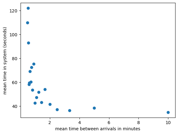
Exercise 5.1
Show code cell source
import numpy as np
import pandas as pd
import random
num_cars=10

k=.1 #mean time between arrivals (in minutes)
df=pd.DataFrame()

#######PROCESS ORDERING DATA#######
df.loc[0,"order_arrival_time"]=0
df.loc[0,"time_to_order"]=15+30*random.uniform(0, 1)
df.loc[0,"pay_arrival_time"]=df.loc[0,"order_arrival_time"] + df.loc[0,"time_to_order"]
df.loc[0,"order_system_time"]=df.loc[0,"pay_arrival_time"]-df.loc[0,"order_arrival_time"]

for i in np.arange(1,num_cars,1):
    df.loc[i,"order_arrival_time"]=df.loc[i-1,"order_arrival_time"]-(60/k)*np.log(1-random.uniform(0, 1))
    df.loc[i,"time_to_order"]=15+30*random.uniform(0, 1)
    df.loc[i,"pay_arrival_time"]=max(df.loc[i,"order_arrival_time"] + df.loc[i,"time_to_order"], df.loc[i-1,"pay_arrival_time"]+df.loc[i,"time_to_order"])
    df.loc[i,"order_system_time"]=df.loc[i,"pay_arrival_time"]-df.loc[i,"order_arrival_time"]

####### PROCESS PAYING DATA #######
if random.uniform(0,1)<.5:
    df.loc[0,"time_to_pay"]=30*random.uniform(0, 1) +5  #pay by cash
else:
    df.loc[0,"time_to_pay"]=15*random.uniform(0, 1)  +5  #pay by credit
df.loc[0,"pickup_arrival_time"]=df.loc[0,"pay_arrival_time"] + df.loc[0,"time_to_pay"]
df.loc[0,"pay_system_time"]=df.loc[0,"pickup_arrival_time"]-df.loc[0,"pay_arrival_time"]

for i in np.arange(1,num_cars,1):
    if random.uniform(0,1)<.5:
        df.loc[i,"time_to_pay"]=30*random.uniform(0, 1)  +5  #pay by cash
    else:
        df.loc[i,"time_to_pay"]=15**random.uniform(0, 1)  +5  #pay by credit
    df.loc[i,"pickup_arrival_time"]=max(df.loc[i,"pay_arrival_time"] + df.loc[i,"time_to_pay"], df.loc[i-1,"pickup_arrival_time"]+df.loc[i,"time_to_pay"] )
    df.loc[i,"pay_system_time"]=df.loc[i,"pickup_arrival_time"]-df.loc[i,"pay_arrival_time"]

###### PROCESS PICKUP DATA #######
df.loc[0,"time_to_pickup"]= 60*random.uniform(0,1)+ 30
df.loc[0,"finish_time"]=df.loc[0,"pickup_arrival_time"] + df.loc[0,"time_to_pickup"]
df.loc[0,"pickup_system_time"]=df.loc[0,"finish_time"]-df.loc[0,"pickup_arrival_time"]

for i in np.arange(1,num_cars,1):
    df.loc[i,"time_to_pickup"]= 60*random.uniform(0,1)+ 30
    df.loc[i,"finish_time"]=max(df.loc[i,"pickup_arrival_time"] + df.loc[i,"time_to_pickup"], df.loc[i-1,"finish_time"]+df.loc[i,"time_to_pickup"] )
    df.loc[i,"pickup_system_time"]=df.loc[i,"finish_time"]-df.loc[i,"pickup_arrival_time"]
table = df[["order_arrival_time","time_to_order","order_system_time","pay_arrival_time","time_to_pay","pay_system_time","pickup_arrival_time","time_to_pickup","pickup_system_time", "finish_time"]]
table
| order_arrival_time | time_to_order | order_system_time | pay_arrival_time | time_to_pay | pay_system_time | pickup_arrival_time | time_to_pickup | pickup_system_time | finish_time | |
|---|---|---|---|---|---|---|---|---|---|---|
| 0 | 0.000000 | 43.602984 | 43.602984 | 43.602984 | 7.556623 | 7.556623 | 51.159607 | 65.477791 | 65.477791 | 116.637398 |
| 1 | 481.388415 | 33.366122 | 33.366122 | 514.754537 | 6.231221 | 6.231221 | 520.985758 | 56.592074 | 56.592074 | 577.577832 |
| 2 | 1219.912249 | 41.477045 | 41.477045 | 1261.389293 | 23.202241 | 23.202241 | 1284.591534 | 58.655755 | 58.655755 | 1343.247289 |
| 3 | 1294.706715 | 30.565060 | 30.565060 | 1325.271775 | 12.672773 | 12.672773 | 1337.944548 | 43.237563 | 48.540305 | 1386.484852 |
| 4 | 1683.852787 | 43.093286 | 43.093286 | 1726.946073 | 6.338934 | 6.338934 | 1733.285006 | 82.937953 | 82.937953 | 1816.222959 |
| 5 | 2240.226570 | 43.522066 | 43.522066 | 2283.748635 | 16.409112 | 16.409112 | 2300.157747 | 51.509599 | 51.509599 | 2351.667346 |
| 6 | 2859.137294 | 39.779653 | 39.779653 | 2898.916947 | 6.035139 | 6.035139 | 2904.952086 | 57.808210 | 57.808210 | 2962.760296 |
| 7 | 4292.462366 | 27.259678 | 27.259678 | 4319.722044 | 23.996465 | 23.996465 | 4343.718509 | 76.043934 | 76.043934 | 4419.762443 |
| 8 | 4423.265534 | 35.461872 | 35.461872 | 4458.727406 | 34.086612 | 34.086612 | 4492.814018 | 76.186779 | 76.186779 | 4569.000797 |
| 9 | 5183.852133 | 22.406112 | 22.406112 | 5206.258245 | 8.030864 | 8.030864 | 5214.289109 | 37.802962 | 37.802962 | 5252.092071 |
Show code cell source
def graph(num_cars,k):
    k=k #mean time between arrivals (in minutes)
    df=pd.DataFrame()

    #######PROCESS ORDERING DATA#######
    df.loc[0,"order_arrival_time"]=0
    df.loc[0,"time_to_order"]=15+30*random.uniform(0, 1)
    df.loc[0,"pay_arrival_time"]=df.loc[0,"order_arrival_time"] + df.loc[0,"time_to_order"]
    df.loc[0,"order_system_time"]=df.loc[0,"pay_arrival_time"]-df.loc[0,"order_arrival_time"]
    for i in np.arange(1,num_cars,1):
        df.loc[i,"order_arrival_time"]=df.loc[i-1,"order_arrival_time"]-(60/k)*np.log(1-random.uniform(0, 1))
        df.loc[i,"time_to_order"]=15+30*random.uniform(0, 1)
        df.loc[i,"pay_arrival_time"]=max(df.loc[i,"order_arrival_time"] + df.loc[i,"time_to_order"], df.loc[i-1,"pay_arrival_time"]+df.loc[i,"time_to_order"])
        df.loc[i,"order_system_time"]=df.loc[i,"pay_arrival_time"]-df.loc[i,"order_arrival_time"]

    ####### PROCESS PAYING DATA #######
    if random.uniform(0,1)<.5:
        df.loc[0,"time_to_pay"]=30*random.uniform(0, 1) +5  #pay by cash
    else:
        df.loc[0,"time_to_pay"]=15*random.uniform(0, 1)  +5  #pay by credit
    df.loc[0,"pickup_arrival_time"]=df.loc[0,"pay_arrival_time"] + df.loc[0,"time_to_pay"]
    df.loc[0,"pay_system_time"]=df.loc[0,"pickup_arrival_time"]-df.loc[0,"pay_arrival_time"]

    for i in np.arange(1,num_cars,1):
        if random.uniform(0,1)<.5:
            df.loc[i,"time_to_pay"]=30*random.uniform(0, 1)  +5  #pay by cash
        else:
            df.loc[i,"time_to_pay"]=15**random.uniform(0, 1)  +5  #pay by credit
        df.loc[i,"pickup_arrival_time"]=max(df.loc[i,"pay_arrival_time"] + df.loc[i,"time_to_pay"], df.loc[i-1,"pickup_arrival_time"]+df.loc[i,"time_to_pay"] )
        df.loc[i,"pay_system_time"]=df.loc[i,"pickup_arrival_time"]-df.loc[i,"pay_arrival_time"]

    ###### PROCESS PICKUP DATA #######
    df.loc[0,"time_to_pickup"]= 60*random.uniform(0,1)+ 30
    df.loc[0,"finish_time"]=df.loc[0,"pickup_arrival_time"] + df.loc[0,"time_to_pickup"]
    df.loc[0,"pickup_system_time"]=df.loc[0,"finish_time"]-df.loc[0,"pickup_arrival_time"]

    for i in np.arange(1,num_cars,1):
        df.loc[i,"time_to_pickup"]= 60*random.uniform(0,1)+ 30
        df.loc[i,"finish_time"]=max(df.loc[i,"pickup_arrival_time"] + df.loc[i,"time_to_pickup"], df.loc[i-1,"finish_time"]+df.loc[i,"time_to_pickup"] )
        df.loc[i,"pickup_system_time"]=df.loc[i,"finish_time"]-df.loc[i,"pickup_arrival_time"]


    system_mean=(np.mean(df["order_system_time"])+np.mean(df["pay_system_time"])+np.mean(df["pickup_system_time"]))/3

    return system_mean
Show code cell source
results=pd.DataFrame()
for n in np.arange(0,20,1):
    k=.1+.1*n
    results.loc[n,"k"]=k
    results.loc[n,"ave_system_time"]=graph(num_cars,k)
Show code cell source
# Graph of k vs ave_system_time
import matplotlib.pyplot as plt

plt.scatter(1/results["k"],results["ave_system_time"])
plt.xlabel("mean time between arrivals in minutes")
plt.ylabel("mean time in system (seconds)")
Text(0, 0.5, 'mean time in system (seconds)')
Note: This type of analysis can be done using an Excel spreadsheet. For example, see https://docs.google.com/spreadsheets/d/1JPq2UfIWMTHizAq6_gH9WYm_qXZodi7v/edit?usp=sharing&ouid=101192945680365451790&rtpof=true&sd=true