import numpy as np
import matplotlib.pyplot as plt
from scipy.integrate import odeint
12.8. Solutions to Exercises#
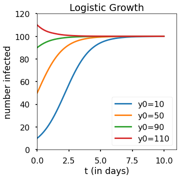
12.8.1. Logistic Growth and COVID-19#
First, separate the variables and antidifferentiate both sides
The partial fraction decomposition
with \(A=1\) and \(B=\frac{1}{kM}\)
leads to
Considering the initial condition \(y(0)=y_0>0\), the solution can be obtained using algebra:
2a)
Show code cell source
import matplotlib.pyplot as plt
import numpy as np
from scipy.integrate import solve_ivp

plt.style.use('seaborn-poster')

%matplotlib inline

k=1
y0a=10
y0b=50
y0c=90
y0d=110
M=100

F = lambda t,y: k*y*(1-y/M)

t_eval = np.arange(0, 10, 0.01)
sola = solve_ivp(F, [0, 10], [y0a], t_eval=t_eval)
solb = solve_ivp(F, [0, 10], [y0b], t_eval=t_eval)
solc = solve_ivp(F, [0, 10], [y0c], t_eval=t_eval)
sold = solve_ivp(F, [0, 10], [y0d], t_eval=t_eval)
plt.figure(figsize = (5,5))
plt.plot(sola.t, sola.y[0])
plt.plot(solb.t, solb.y[0])
plt.plot(solc.t, solc.y[0])
plt.plot(sold.t, sold.y[0])


plt.title('Logistic Growth')
plt.xlabel('t (in days)')
plt.ylabel('number infected')
plt.ylim((0,120))
plt.xlim((0,11))
plt.legend(['y0=10','y0=50','y0=90','y0=110'])
plt.show()
<ipython-input-1-b136c51ef48b>:5: MatplotlibDeprecationWarning: The seaborn styles shipped by Matplotlib are deprecated since 3.6, as they no longer correspond to the styles shipped by seaborn. However, they will remain available as 'seaborn-v0_8-<style>'. Alternatively, directly use the seaborn API instead.
  plt.style.use('seaborn-poster')
2b)
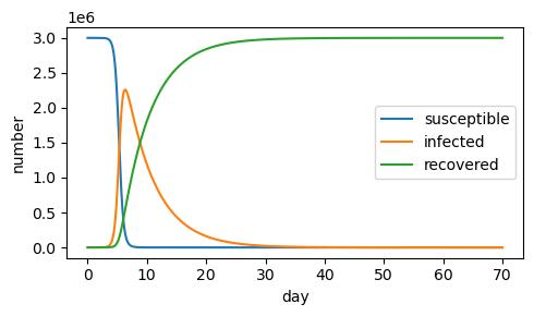
12.8.2. The Basic SIR Model#
Exercise 1
a) If the initial population is increased to 3,000,000, the epidemic appears to end sooner (around day 30)
Show code cell source
import numpy as np
import matplotlib.pyplot as plt
from scipy.integrate import odeint

# Define Equations
def f(y, t, params):
    S, I, R = y      # unpack current values of y
    beta, gamma      # unpack parameters
    #specify dS/dt, dI/dt and dR/dt
    derivs = [-beta * S * I,
             beta * S * I - gamma * I,
             gamma * I]
    return derivs

# Parameters
beta=.000001
gamma=.2
# Initial values
S0=3000000
I0=1
R0=0

# Bundle parameters for ODE solver
params = [beta,gamma]
# Bundle initial conditions for ODE solver
y0 = [S0,I0,R0]

# Make time array for solution
tStop = 70  # number of days
tInc = .001
t = np.arange(0., tStop, tInc)

# Call the ODE solver
psoln = odeint(f, y0, t, args=(params,))

# Plot results
fig = plt.figure(1, figsize=(5,3))
plt.plot(t, psoln[:,0],label='susceptible')
plt.plot(t, psoln[:,1],label='infected')
plt.plot(t, psoln[:,2],label='recovered')
plt.legend()
plt.xlabel('day')
plt.ylabel('number')
plt.savefig("SIR.png")
plt.tight_layout()
plt.show()
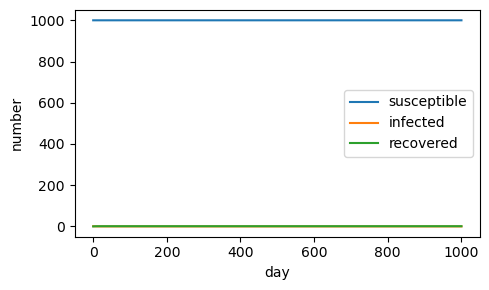
If the initial population is reduced to 1,000, there is no epidemic.
Show code cell source
import numpy as np
import matplotlib.pyplot as plt
from scipy.integrate import odeint

# Define Equations
def f(y, t, params):
    S, I, R = y      # unpack current values of y
    beta, gamma      # unpack parameters
    #specify dS/dt, dI/dt and dR/dt
    derivs = [-beta * S * I,
             beta * S * I - gamma * I,
             gamma * I]
    return derivs

# Parameters
beta=.000001
gamma=.2
# Initial values
S0=1000
I0=1
R0=0

# Bundle parameters for ODE solver
params = [beta,gamma]
# Bundle initial conditions for ODE solver
y0 = [S0,I0,R0]

# Make time array for solution
tStop = 1000  # number of days
tInc = .001
t = np.arange(0., tStop, tInc)

# Call the ODE solver
psoln = odeint(f, y0, t, args=(params,))

# Plot results
fig = plt.figure(1, figsize=(5,3))
plt.plot(t, psoln[:,0],label='susceptible')
plt.plot(t, psoln[:,1],label='infected')
plt.plot(t, psoln[:,2],label='recovered')
plt.legend()
plt.xlabel('day')
plt.ylabel('number')
plt.savefig("SIR.png")
plt.tight_layout()
plt.show()
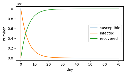
b) If the transmission rate is high (\(\beta=.0001\)), the entire population is quickly infected, and the epidemic ends sooner (around day 20).
Show code cell source
import numpy as np
import matplotlib.pyplot as plt
from scipy.integrate import odeint

# Define Equations
def f(y, t, params):
    S, I, R = y      # unpack current values of y
    beta, gamma      # unpack parameters
    #specify dS/dt, dI/dt and dR/dt
    derivs = [-beta * S * I,
             beta * S * I - gamma * I,
             gamma * I]
    return derivs

# Parameters
beta=.0001
gamma=.2
# Initial values
S0=1000000
I0=1
R0=0

# Bundle parameters for ODE solver
params = [beta,gamma]
# Bundle initial conditions for ODE solver
y0 = [S0,I0,R0]

# Make time array for solution
tStop = 70  # number of days
tInc = .001
t = np.arange(0., tStop, tInc)

# Call the ODE solver
psoln = odeint(f, y0, t, args=(params,))

# Plot results
fig = plt.figure(1, figsize=(5,3))
plt.plot(t, psoln[:,0],label='susceptible')
plt.plot(t, psoln[:,1],label='infected')
plt.plot(t, psoln[:,2],label='recovered')
plt.legend()
plt.xlabel('day')
plt.ylabel('number')
plt.savefig("SIR.png")
plt.tight_layout()
plt.show()
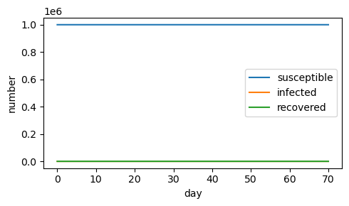
If the infection rate is reduced (\(\beta=10^{-7}\)), there is no epidemic.
Show code cell source
import numpy as np
import matplotlib.pyplot as plt
from scipy.integrate import odeint

# Define Equations
def f(y, t, params):
    S, I, R = y      # unpack current values of y
    beta, gamma      # unpack parameters
    #specify dS/dt, dI/dt and dR/dt
    derivs = [-beta * S * I,
             beta * S * I - gamma * I,
             gamma * I]
    return derivs

# Parameters
beta=.0000001
gamma=.2
# Initial values
S0=1000000
I0=1
R0=0

# Bundle parameters for ODE solver
params = [beta,gamma]
# Bundle initial conditions for ODE solver
y0 = [S0,I0,R0]

# Make time array for solution
tStop = 70  # number of days
tInc = .001
t = np.arange(0., tStop, tInc)

# Call the ODE solver
psoln = odeint(f, y0, t, args=(params,))

# Plot results
fig = plt.figure(1, figsize=(5,3))
plt.plot(t, psoln[:,0],label='susceptible')
plt.plot(t, psoln[:,1],label='infected')
plt.plot(t, psoln[:,2],label='recovered')
plt.legend()
plt.xlabel('day')
plt.ylabel('number')
plt.savefig("SIR.png")
plt.tight_layout()
plt.show()
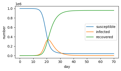
c) If the recovery rate is increased (\(\gamma=.3\)), fewer people get infected.
Show code cell source
import numpy as np
import matplotlib.pyplot as plt
from scipy.integrate import odeint

# Define Equations
def f(y, t, params):
    S, I, R = y      # unpack current values of y
    beta, gamma      # unpack parameters
    #specify dS/dt, dI/dt and dR/dt
    derivs = [-beta * S * I,
             beta * S * I - gamma * I,
             gamma * I]
    return derivs

# Parameters
beta=.000001
gamma=.3
# Initial values
S0=1000000
I0=1
R0=0

# Bundle parameters for ODE solver
params = [beta,gamma]
# Bundle initial conditions for ODE solver
y0 = [S0,I0,R0]

# Make time array for solution
tStop = 70  # number of days
tInc = .001
t = np.arange(0., tStop, tInc)

# Call the ODE solver
psoln = odeint(f, y0, t, args=(params,))

# Plot results
fig = plt.figure(1, figsize=(5,3))
plt.plot(t, psoln[:,0],label='susceptible')
plt.plot(t, psoln[:,1],label='infected')
plt.plot(t, psoln[:,2],label='recovered')
plt.legend()
plt.xlabel('day')
plt.ylabel('number')
plt.savefig("SIR.png")
plt.tight_layout()
plt.show()
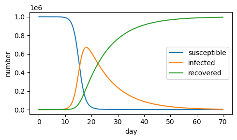
If the recovery rate is decreased (\(\gamma=.1\)), more people get infected, and the epidemic persists over a longer number of days.
Show code cell source
import numpy as np
import matplotlib.pyplot as plt
from scipy.integrate import odeint

# Define Equations
def f(y, t, params):
    S, I, R = y      # unpack current values of y
    beta, gamma      # unpack parameters
    #specify dS/dt, dI/dt and dR/dt
    derivs = [-beta * S * I,
             beta * S * I - gamma * I,
             gamma * I]
    return derivs

# Parameters
beta=.000001
gamma=.1
# Initial values
S0=1000000
I0=1
R0=0

# Bundle parameters for ODE solver
params = [beta,gamma]
# Bundle initial conditions for ODE solver
y0 = [S0,I0,R0]

# Make time array for solution
tStop = 70  # number of days
tInc = .001
t = np.arange(0., tStop, tInc)

# Call the ODE solver
psoln = odeint(f, y0, t, args=(params,))

# Plot results
fig = plt.figure(1, figsize=(5,3))
plt.plot(t, psoln[:,0],label='susceptible')
plt.plot(t, psoln[:,1],label='infected')
plt.plot(t, psoln[:,2],label='recovered')
plt.legend()
plt.xlabel('day')
plt.ylabel('number')
plt.savefig("SIR.png")
plt.tight_layout()
plt.show()
d) As we saw in part b), with a high enough transmission rate, the entire population can become infected.
e) As we also saw in part b), with a low enough transmission rate, there is no outbreak.
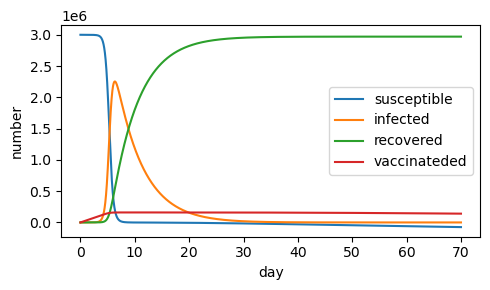
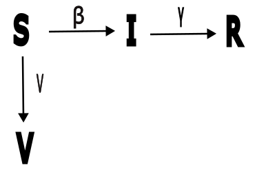
Exercise 2
Show code cell source
import numpy as np
import matplotlib.pyplot as plt
from scipy.integrate import odeint

# Define Equations
def SIRV(y, t, params):
    S, I, R, V = y      # unpack current values of y
    beta, gamma, v     # unpack parameters
    #specify dS/dt, dI/dt and dR/dt
    derivs = [-beta * S * I - v*V,
             beta * S * I - gamma * I,
             gamma * I,
             v*S]
    return derivs

# Parameters
beta=.000001
gamma=.2
v=.01
# Initial values
S0=3000000
I0=1
R0=0
V0=0

# Bundle parameters for ODE solver
params = [beta,gamma,v]
# Bundle initial conditions for ODE solver
y0 = [S0,I0,R0,V0]

# Make time array for solution
tStop = 70  # number of days
tInc = .001
t = np.arange(0., tStop, tInc)

# Call the ODE solver
psoln = odeint(SIRV, y0, t, args=(params,))

# Plot results
fig = plt.figure(1, figsize=(5,3))
plt.plot(t, psoln[:,0],label='susceptible')
plt.plot(t, psoln[:,1],label='infected')
plt.plot(t, psoln[:,2],label='recovered')
plt.plot(t, psoln[:,3],label='vaccinateded')
plt.legend()
plt.xlabel('day')
plt.ylabel('number')
plt.savefig("SIRV.png")
plt.tight_layout()
plt.show()
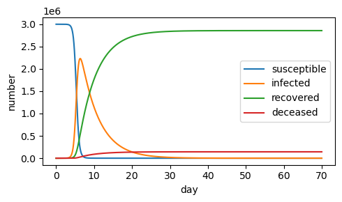
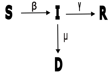
Exercise 3
Show code cell source
import numpy as np
import matplotlib.pyplot as plt
from scipy.integrate import odeint

# Define Equations
def SIRD(y, t, params):
    S, I, R, D= y      # unpack current values of y
    beta, gamma, mu     # unpack parameters
    #specify dS/dt, dI/dt and dR/dt
    derivs = [-beta * S * I,
             beta * S * I - gamma * I - mu*I,
             gamma * I,
             mu*I]
    return derivs

# Parameters
beta=.000001
gamma=.2
mu=.01
# Initial values
S0=3000000
I0=1
R0=0
D0=0

# Bundle parameters for ODE solver
params = [beta,gamma,mu]
# Bundle initial conditions for ODE solver
y0 = [S0,I0,R0,D0]

# Make time array for solution
tStop = 70  # number of days
tInc = .001
t = np.arange(0., tStop, tInc)

# Call the ODE solver
psoln = odeint(SIRD, y0, t, args=(params,))

# Plot results
fig = plt.figure(1, figsize=(5,3))
plt.plot(t, psoln[:,0],label='susceptible')
plt.plot(t, psoln[:,1],label='infected')
plt.plot(t, psoln[:,2],label='recovered')
plt.plot(t, psoln[:,3],label='deceased')
plt.legend()
plt.xlabel('day')
plt.ylabel('number')
plt.savefig("SIRD.png")
plt.tight_layout()
plt.show()
12.8.3. Cholera in Haiti#
Exercise 1
Show code cell source
import numpy as np
import matplotlib.pyplot as plt
from scipy.integrate import odeint

# Define Equations
def f(y, t, params):
    S, I, B = y      # unpack current values of y
    H,n,a,K,r,Nb,e      # unpack parameters
    #specify dS/dt, dI/dt and dR/dt
    derivs = [n*(H-S)-a*B*S/(K+B),
             a*B*S/(K+B)-r*I,
             B*Nb+e*I]
    return derivs

# Parameters
H=10000
n=.0001
K=10**6
r=.2
Nb=-.33
e=10
# Initial values
S0=10000
I0=100
B0=0

exposure_rate=[]
max_infected=[]

for a in np.arange(0,100,1):
    exposure_rate.append(a)
    # Bundle parameters for ODE solver
    params = [H,n,a,K,r,Nb,e]
    # Bundle initial conditions for ODE solver
    y0 = [S0,I0,B0]

    # Make time array for solution
    tStop = 10  # number of days
    tInc = .001
    t = np.arange(0., tStop, tInc)

    # Call the ODE solver
    psoln = odeint(f, y0, t, args=(params,))
    max_infected.append(np.max(psoln[:,1]))

# Plot results
fig = plt.figure(1, figsize=(5,3))
plt.plot(exposure_rate, max_infected,label='max infected')
plt.legend()
plt.xlabel('a=exposure rate')
plt.ylabel('max infected population')
plt.savefig("cholerEx1.png")
plt.tight_layout()
plt.show()
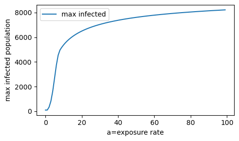
The max infected population rises sharply as the exposure rate (a) is increased from 0 to 10. When a=100, the max_infected population has leveled off at approximately 8000 people.
Exercise 2
Show code cell source
import numpy as np
import matplotlib.pyplot as plt
from scipy.integrate import odeint

# Define Equations
def f(y, t, params):
    S, I, B = y      # unpack current values of y
    H,n,a,K,r,Nb,e      # unpack parameters
    #specify dS/dt, dI/dt and dR/dt
    derivs = [n*(H-S)-a*B*S/(K+B),
             a*B*S/(K+B)-r*I,
             B*Nb+e*I]
    return derivs

# Parameters
H=10000
n=.0001
K=10**6
r=.2
Nb=-.33
# Initial values
S0=10000
I0=100
B0=0

contam=[]
peak1=[]
peak2=[]

for e in np.arange(0,50,1):
    contam.append(e)
    a=40
    # Bundle parameters for ODE solver
    params = [H,n,a,K,r,Nb,e]
    # Bundle initial conditions for ODE solver
    y0 = [S0,I0,B0]

    # Make time array for solution
    tStop = 10  # number of days
    tInc = .001
    t = np.arange(0., tStop, tInc)

    # Call the ODE solver
    psoln = odeint(f, y0, t, args=(params,))
    peak1.append(np.max(psoln[:,1]))

    a=20
        # Bundle parameters for ODE solver
    params = [H,n,a,K,r,Nb,e]
    # Bundle initial conditions for ODE solver
    y0 = [S0,I0,B0]

    # Make time array for solution
    tStop = 10  # number of days
    tInc = .001
    t = np.arange(0., tStop, tInc)

    # Call the ODE solver
    psoln = odeint(f, y0, t, args=(params,))
    peak2.append(np.max(psoln[:,1]))

# Plot results
fig = plt.figure(1, figsize=(5,3))
plt.plot(contam, peak1,label='max infected (a=40)')
plt.plot(contam, peak2,label='max infected (a=20)')
plt.legend(["a=40","a=20"])
plt.xlabel('e=water contamination rate')
plt.ylabel('max infected population')
plt.savefig("cholerEx2.png")
plt.tight_layout()
plt.show()
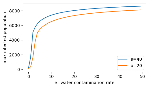
Increased exposure rate (a=20 to a=40) increases the max infected population at each level of the water contamination rate (e).
Exercise 3
Show code cell source
import numpy as np
import matplotlib.pyplot as plt
from scipy.integrate import odeint

# Define Equations
def f(y, t, params):
    S, I, B = y      # unpack current values of y
    H,n,a,K,r,Nb,e      # unpack parameters
    #specify dS/dt, dI/dt and dR/dt
    derivs = [n*(H-S)-a*B*S/(K+B),
             a*B*S/(K+B)-r*I,
             B*Nb+e*I]
    return derivs

# Parameters
H=10000
n=.0001
K=10**6
e=10
Nb=-.33
# Initial values
S0=10000
I0=100
B0=0

recovery=[]
peak1=[]
peak2=[]

for r in np.arange(0,.8,.01):
    recovery.append(r)
    a=40
    # Bundle parameters for ODE solver
    params = [H,n,a,K,r,Nb,e]
    # Bundle initial conditions for ODE solver
    y0 = [S0,I0,B0]

    # Make time array for solution
    tStop = 10  # number of days
    tInc = .001
    t = np.arange(0., tStop, tInc)

    # Call the ODE solver
    psoln = odeint(f, y0, t, args=(params,))
    peak1.append(np.max(psoln[:,1]))

    a=80
        # Bundle parameters for ODE solver
    params = [H,n,a,K,r,Nb,e]
    # Bundle initial conditions for ODE solver
    y0 = [S0,I0,B0]

    # Make time array for solution
    tStop = 10  # number of days
    tInc = .001
    t = np.arange(0., tStop, tInc)

    # Call the ODE solver
    psoln = odeint(f, y0, t, args=(params,))
    peak2.append(np.max(psoln[:,1]))

# Plot results
fig = plt.figure(1, figsize=(5,3))
plt.plot(recovery, peak1,label='max infected (a=40)')
plt.plot(recovery, peak2,label='max infected (a=80)')
plt.xlabel('r=recovery rate')
plt.ylabel('max infected population')
plt.savefig("cholerEx3.png")
plt.tight_layout()
plt.show()
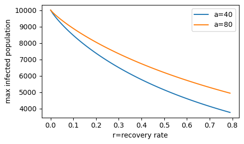
Peak infection dependency on the cholera recovery rate r for two exposure levels (a=40/day and a=80/day).
Exercise 4
Show code cell source
import numpy as np
import matplotlib.pyplot as plt
from scipy.integrate import odeint
# Define Equations
def f(y, t, params):
S, I, B = y # unpack current values of y
H,n,a,K,r,Nb,e # unpack parameters
#specify dS/dt, dI/dt and dR/dt
derivs = [n*(H-S)-a*B*S/(K+B),
a*B*S/(K+B)-r*I,
B*Nb+e*I]
return derivs
# Parameters
H=10000
n=.0001
K=10**6
r=.2
e=10
Nb=-.33
# Initial values
S0=10000
I0=0
Z=np.eye(101, 201)
for B0 in np.arange(0,100,1):
for i in np.arange(0,200,1):
a=i/10 # exposure rate
# Bundle parameters for ODE solver
params = [H,n,a,K,r,Nb,e]
# Bundle initial conditions for ODE solver
y0 = [S0,I0,B0]
# Make time array for solution
tStop = 10 # number of days
tInc = .001
t = np.arange(0., tStop, tInc)
# Call the ODE solver
psoln = odeint(f, y0, t, args=(params,))
# Record the peak infection
Z[B0,i]=np.max(psoln[:,1])
# Plot results
# Creating dataset
x=np.arange(0,100,1)
y=np.arange(0,200,1)
# Creating figure
fig = plt.figure()
# syntax for 3-D projection
ax = plt.axes(projection ='3d')
for i in np.arange(1,100,1):
for j in np.arange(0,200,1):
ax.scatter(i, j, Z[i,j],color='lightgray')
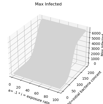
ax.set_title('Max Infected')
ax.set_xlabel('a= .1 * i = exposure rate')
ax.set_ylabel('B0=initial bacteria concent')
ax.set_zlabel('Max Infected')
plt.savefig("cholerEx4.png")
plt.show()
Exercise 5
a) Though it would be better to revise the model by adding a vaccinated compartment V (t), the basic model might reflect a vaccination program by lowering the initial susceptible population S(0) and raising the value of K, the latter being the bacteria concentration required to give a .5 probability.
b) Seasonal behavior of cholera outbreaks which may be related to weather events such as floods or El Nino must be considered. That is, even though there may be a period with no or very few cases, there is a latent possibility for re-emergence of a large number of infected population. Mathematically viable solutions may be overly simplistic in light of the reality of everyday life in Haiti.
From the sensitivity analysis, the contamination rate seems to have the largest effect on the infected population, although exposure rate, recovery rate, and initial concentration of bacteria also have an effect. Within the range of 2.5-30 number of people contaminated per day, the infected population will increase significantly. As the contamination rate increases above 30, the infected population stabilizes and increases more slowly. These observations suggest focusing response and preparation measures on lowering the contamination rate
12.8.4. CWS Model of Alzheimer’s Disease#
Exercise 1
Exercise 2
The total exit rate of monomers from the CSF (\(h_2=r_{21}+r_{23}+L_2\)) is the sum of the respective rates monomers move from the CSF to the brain (\(r_{21}\) and from CSF to plasma (\(r_{23}\)), these being added to the loss of monomers in the brain by degradation (\(L_2\)).
Exercises 3
Treatment 2 shows that the plasma and CSF levels of amyloid-beta monomers might increase, but the level in the brain actually decreases.
Exercise 4
Show code cell source
import numpy as np
import matplotlib.pyplot as plt
from scipy.integrate import odeint

def f(y, t, params):
    b1, c,p = y      # unpack current values of y
    k1,k2,k3, r12,r13,r23,r21,r31,r32,L1,L2,L3,E,F,S = params  # unpack parameters
    derivs = [k1+F*S+r31*p+r21*c-(r13*b1+r12*b1*(1+np.heaviside(t-100,0)-np.heaviside(t-465,0)))-(L1+E*S)*b1-2*E*b1**2,      # list of dy/dt=f functions
             k2+r12*b1*(1+np.heaviside(t-100,0)-np.heaviside(t-465,0))+r32*p-(r21*c+r23*c)-L2*c,
             k3+r13*b1+r23*c-(r31*p+r32*p)-L3*p]
    return derivs

# Parameters
k1 = 7.34*86400
L1 = 24
k2=0
L2=0
k3=0
L3=6.7*10**(-3)*86400
r12=7.6*10**(-6)*86400
r23=1.7*10**(-3)*86400
r31=3.7*10**(-5)*86400
r32=0
r21=0
r13=0
E=0
F=.238
S=0

# Initial values
b10 = 25.7*(10**3)
c0 = 115
p0 = 29

# Bundle parameters for ODE solver
params = [k1,k2,k3, r12,r13,r23,r21,r31,r32,L1,L2,L3,E,F,S]

# Bundle initial conditions for ODE solver
y0 = [b10,c0,p0]

# Make time array for solution
tStop = 1000
tInc = 0.05
t = np.arange(0., tStop, tInc)

# Call the ODE solver
psoln = odeint(f, y0, t, args=(params,))

# Plot results
fig = plt.figure(1, figsize=(8,8))

# Plot b1 as a function of time
ax1 = fig.add_subplot(311)
ax1.plot(t, psoln[:,0])
ax1.set_xlabel('time')
ax1.set_ylabel('b1')

# Plot c as a function of time
ax2 = fig.add_subplot(312)
ax2.plot(t, psoln[:,1])
ax2.set_xlabel('time')
ax2.set_ylabel('c')

# Plot p as a function of time
ax3 = fig.add_subplot(313)
ax3.plot(t, psoln[:,2])
ax3.set_xlabel('time')
ax3.set_ylabel('p')
plt.savefig("treatment2nonlin.png")
plt.tight_layout()
plt.show()

The output of the nonlinear is the same as the simplified linear model since the former is equivalent to the latter when \(E=S=0\).
12.8.5. Gravity-Fed Water Delivery#
[2.1] \(F_{gn}=F_{g} \cos(\theta) = \gamma \delta V \cos(\theta) = \gamma \delta V \sqrt{1-(\frac{dz}{ds})^2}\).
[2.2] \(\frac{dp}{ds}\approx \frac{p(s_0-\frac{\delta s}{2})-p(s_0)}{-\frac{\delta s}{2}} \Rightarrow p(s_0-\frac{\delta s}{2}) \approx p(s_0) - \frac{dp}{ds} \frac{\delta s}{2}\).
[2.3] Since \(z\) has dimension \(L\), we must show the other two terms do as well. Pressure being force per unit area, and force being mass time acceleration, \(p\) has dimension \(\frac{M \frac{L}{T^2} }{L^2}=\frac{M}{LT^2}\). Since \(\gamma=\rho g\) has dimension \(\frac {M}{L^3} \frac{L}{T^2} = \frac{M}{L^2T^2}\), the dimension of \(\frac{p}{\gamma}\) is \(\frac{M}{LT^2} \frac{L^2T^2}{M}=L\). The dimension for \(\frac{u^2}{g}\) is \(\frac{(\frac{L}{T})^2}{\frac{L}{T^2}}=L\).
[3.1.1]
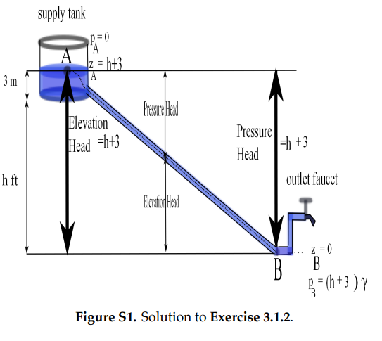
[a] Bernoulli’s equation states \(\frac{p}{\gamma}\) + \(\frac{u^2}{2g}\) + z = c. Since \(u=0\) \(\frac{m}{sec}\) as a result of the tap being closed, \(z_B=0\) m as shown in {\bf Figure \ref{fig9}}, and so our equation simplifies to \(\frac{p}{\gamma}\) = c. Observing that c = 9 m + 2 m = 11 ft = \(\frac{p \frac{kN}{m^2} }{9.789{\frac{kN}{m^3}}}\), we obtain \(p = 105.5\) \({\frac{kN}{m^2}}\).
[b] From part a we know \(\frac{p}{\gamma}\) = c. Observing that c = 30 ft + 6 ft = 36 ft = \(\frac{p \frac{lb}{ft^2} }{62.3 {\frac{lb}{ft^3}}}\), we obtain \(p = 2242.8\) \({\frac{lb}{ft^2}} = 2242.8 {\frac{lb}{ft^2}} \cdot {\frac{(1 ft)^2}{(12 in)^2}} = 15.6 {\frac{lb}{in^2}}\).
[3.1.2] Referring to Figure (S1), let \(h\) be the desired vertical distance from the source reservoir to the faucet. Then \(h\) satisfies
[3.2.1] [a] At a horizontal distance of 600 m, pressure is greatest since the vertical drop from the source is a maximum (114 m).
[b] The pipe can operate at a pressure head of \(\frac{p}{\gamma}=\frac{917 \frac{kN}{m^2}}{9.789\frac{kN}{m^3}}\) = 93.7 m, so 1 intermediate tank is required.
[3.2.2] Pressure at A is equal to \(p_A=[(h_1+h_2)-(h_3+h_4)]\gamma\). The pressure at B is equal to \(p_B=(h_3+h_4)\gamma\). The break-pressure tank effectively reduces the pressure at the faucet by the amount \(p_A\).
[3.3.1] .1215 liters/sec.
[3.3.2] [a] A velocity head of 3 m (10 ft) corresponds to a speed \(u_1=[3(2)(9.8)]^{1/2}\approx 7.7\) m/s. By the continuity equation, \(\pi (0.025)^2 u_1 = \pi (0.02)^2 u_2\) so \(u_2 \approx 11.9\) m/s with a corresponding velocity head of roughly 7.3 m (31.6 feet).
[b]
[4.1]
A negative pressure means that pressure inside the pipe is less than outside. This can cause dirt or air to be sucked into the pipe, resulting in a stoppage of flow.
[4.2] The Reynolds number \(\frac{\rho \bar{u} D}{\mu}\) is dimensionless since all units cancel in the expression \(\frac{\frac{M}{L^3}\frac{L}{T}L}{\frac{M}{LT}}\).
[4.3.1] \(F_{gs} = - F_g \sin \theta = - m g \sin \theta = - \rho (\pi r^2 L) g \sin \theta = - \gamma \pi r^2 L \sin \theta.\)
[4.3.2] \(Q = \int_0^{2\pi} \int_0^R u_0(1-(r/R)^2 ) r dr d\theta = \frac{\pi R^2 u_0}{2}\).
[4.3.3] Since the pipe is wider at B than at A, \(u_B\) is less than \(u_A\). Head loss from A to B is represented by \(h_{AB}\).
[4.3.4] $\( Re=\frac{\rho \bar{u} D}{\mu}=\frac{998.2\cdot 2\cdot D}{0.001}<2100\Rightarrow D<0.001 m = 1 mm. \)$
The flow rate would be
So for a very reasonable \(\bar{u}\) the pipe would have to be unreasonably small. This shows that, while laminar flow is a useful assumption to analyze friction, it is unrealistic for gravity-fed water delivery systems.
[4.4.1] The iron pipe has the greater friction factor.
[4.4.2]
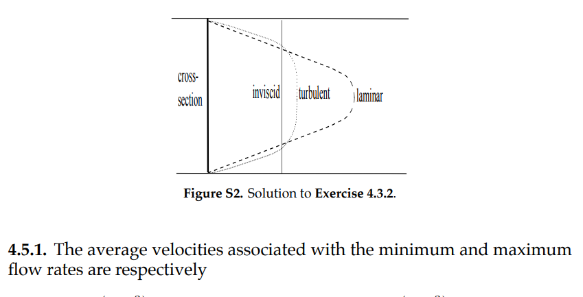
[4.5.1] The average velocities associated with the minimum and maximum flow rates are respectively \(\stackrel{-}{u} = .35 \frac{(10^{-3})}{\pi (.0125)^2} =.71 (m/s)\) and \(\stackrel{-}{u} = 1.4 \frac{(10^{-3})}{\pi (.0125)^2} = 2.85\) (m/s). The respective Reynolds numbers are \(Re = \frac{1.23(.71)(.025)}{1.79(10^{-5})} \approx 1200\), and \(Re = \frac{1.23(2.85)(.025)}{1.79(10^{-5})} \approx 4900.\) This indicates that the flow at the minimum flow rate is laminar, but will be turbulent at the maximum flow rate. Note in {\bf Table 5} the big difference in head loss between these laminar and turbulent flows: 3.45 m per 100 m at the minimum flow rate versus 49.5 m per 100 m at the maximum flow rate.
[4.5.2] Using the equation for \(f\) given in {\bf (\ref{Colebrook})} or a Moody chart , we can determine the Reynolds number \(Re\). We may then compute
and
Knowing the head loss, we can easily plot the HGL on the graph shown in Figure (21). The HGL will help us decide whether the pipe may be used for that segment of the system as explained in Section 4.4.
[5.1] There are different possible designs, but a system using a 80 mm diameter is shown here. In 10 years Tesuque Pueblo will have about 1148 people and a required volumetric flow rate of \(Q=4.27 l/s=0.00427 m^3/s\). A 80 mm diameter pipe has a cross-sectional area of 0.005 \(m^2\), so our average velocity is 0.85 m/s (low, but within limits). The maximum static pressure will be \(2255-1950=335\) m at the outlet faucet, which is above the maximum operating pressure head from {\bf Table 5} (146 m). Break pressure tanks at elevations of 2130 m and 2030 m reduce the maximum static pressures to 125 m, 100 m, and 110 m in the first, second, and third sections, respectively (Note that since a 2030 m elevation isn’t included in the survey, we don’t know if there is a suitable building site at this location. In that case a third break pressure tank would be needed). By rounding our flow rate down we get from {\bf Table 5} a head loss of about 0.96 m per 100 m. We will approximate horizontal distance as pipe length, so our HGL is modeled by the equation \(2255-\frac{0.85^2}{2g}-0.96x\). If we compare this line to the given elevations we find the elevations remain below the HGL line. This means the dynamic pressure will never be negative and the system is feasible.
12.8.6. Earthquake Resistant Construction#
2.1
a) \(u=c_1 \cos t + c_2 \sin t\);
b) \(u(t)=e^{-\frac{1}{2}t}[ c_1 \cos( \frac{\sqrt{3}}{2} t )+ c_2 \sin( \frac{\sqrt{3}}{2} t ) ]\);
c)\(u(t)=e^{-t}(c_1+ c_2 t)\);
d) \(u(t)= c_1 e^{(-2+\sqrt{3})t}+c_2e^{(-2-\sqrt{3})t}\).
2.2 For example, to check the solution for \(c=4\), the initial conditions \(u(0)=1\), \(\stackrel{.}{u}(0)=0\) imply that the constants \(c_1\) and \(c_2\) in the general solution \(u(t)= c_1 e^{(-2+\sqrt{3})t}+c_2e^{(-2-\sqrt{3})t}\) must satisfy
It follows easily that \(c_1=\frac{2+\sqrt{3}}{2\sqrt{3}}\) and \(c_2=\frac{-2+\sqrt{3}}{2\sqrt{3}}\).
2.3 For \(0<c<4\), \(u=h_h+u_p\) where \(u_h\) satisfies
and \(u_p=A\cos(2t)+B\sin(2t)\) is a particular solution to the non-homogeneous equation. Solving, we have \(u=\frac{1}{2c} \sin(2t) - \frac{2}{c\sqrt{16-c^2}}e^{\frac{-ct}{2}}\sin(\frac{\sqrt{16-c^2}}{2}t).\)
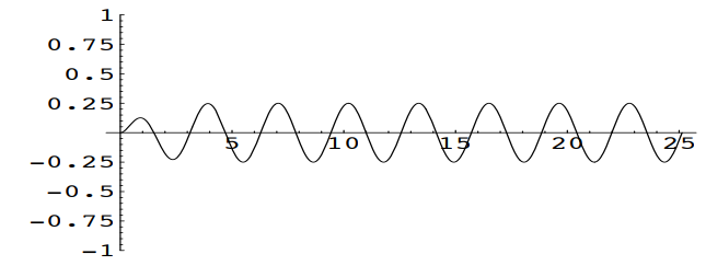
At the critical value \(c=4\), the solution becomes \(u=-\frac{1}{4}te^{-2t} + \frac{1}{8} \sin(2t)\)
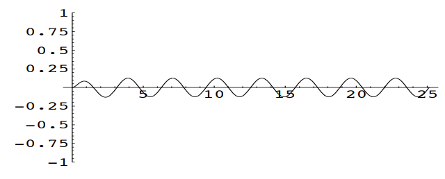
Note that in general, increasing the damping coefficient \(c\) will reduce the amplitude of the periodic term \(\frac{1}{2c} \sin(2t)\) in the solution and cause a more rapid decay of the transient term \(\frac{2}{c\sqrt{16-c^2}}e^{\frac{-ct}{2}}\sin(\frac{\sqrt{16-c^2}}{2}t)\) in the solution.
2.4 Since \(Rmax=2=\frac{k umax}{Fmax}\) with \(k=10^{10} \frac{kg}{sec}\) and \(umax=5\)x\(10^{-3}\), we obtain the maximum allowable blast force \(Fmax= 2.5(10^7) N.\)
2.4.1
2.4.2 a)
b) $\( L[u]=\frac{Fmax}{m}\{\frac{\frac{-1}{T}+s}{s^2(s^2+\omega_0^2)}+\frac{\frac{1}{T}+e^{-Ts}}{s^2(s^2+\omega_0^2)}\} \)$
c)
2.5 The ground motion \(z(t)\) effectively creates a reversed inertial force \(- m \stackrel{..}{z}\).
3.1 \(W=\left(\begin{array}{c}w_1\\w_2\\w_3 \end{array}\right)\) represents the relative displacements, \(M=\left(\begin{array}{ccc}m_1&0&0\\0&m_2&0\\0&0&m_3\end{array}\right)\) represents the mass of the floors, \(K=\left(\begin{array}{ccc}2(k_1+k_2)&-2k_2&0\\-2k_2&2(k_2+k_3)&-2k_3\\0&-2k_3&2k_3\end{array}\right)\) represents the spring constants, and \(F=\left(\begin{array}{c}F_1-m_1\stackrel{..}{z}\\F_2- m_2\stackrel{..}{z}\\F_3- m_3\stackrel{..}{z}\end{array}\right)\) the represents wind force and the inertial force caused by the ground motion.
3.3 \(x_1(t)=\frac{6+2\sqrt{17}}{5\sqrt{17}+17}+c_{11} \cos \sqrt{ \frac{5+\sqrt{17}}{4}} t + c_{12} \sin \sqrt{ \frac{5+\sqrt{17}}{4}} t\) and \(x_2(t)= \frac{-6+2\sqrt{17}}{5\sqrt{17}-17} + c_{21} \cos \sqrt{ \frac{5-\sqrt{17}}{4}} t + c_{22} \sin \sqrt{ \frac{5-\sqrt{17}}{4}} t \). The initial conditions \(w_1(0)=w_2(0)= \stackrel{.}{w_1}(0)= \stackrel{.}{w_2}(0)=0\) imply that \(x_1(0)=x_2(0)=\stackrel{.}{x_1}=(0)= \stackrel{.}{x_2}(0)=0\), giving \(c_{11}= \frac{-6-2\sqrt{17}}{5\sqrt{17}+17} ,c_{12}= 0, c_{22}= \frac{6-2\sqrt{17}}{5\sqrt{17}-17}, c_{21}= 0\). Finally, using \(W= \Phi X\) gives \(w_1(t)= x_1(t)+x_2(t)\), and \(w_2(t)= (\frac{3-\sqrt{17}}{4})x_1(t) + (\frac{3+\sqrt{17}}{4})x_2(t) \).
3.4 \(U=\left[ \begin{array}{c} u(t)\\ \theta(t) \end{array} \right]\), \(M=\left[ \begin{array}{cc} M+m&Ma\\ Ma&I_G+Ma^2 \end{array} \right]\) , \(C=\left[ \begin{array}{cc} c&0\\ 0&0 \end{array} \right]\), \(K=\left[ \begin{array}{cc} k&0\\ 0&K-Mga \end{array} \right]\) and \( F(t) =\left[ \begin{array}{c} c\stackrel{.}{z}+kz \\ 0 \end{array} \right] \)