8.4. Derivatives

Note

Below is the list of topics that are covered in this section:

• Derivatives and Derivative Notations

• Properties, Formulas, and Rules

• Derivative Graphs

• Extrema

• The Mean Value Theorem

• Linearization

• Implicit Differentiation

import sympy as sp
import numpy as np
import matplotlib.pyplot as plt

8.4.1. Derivatives and Derivative Notations

Derivative shows the sensitivity of change of a function’s output when the input changes.
From the previous section, this is the same as what is being measured by the instantaneous rate of change (RoC), which is the slope of the tangent line at a certain point.
One notation of the derivative of the function \(f(x)\) is \(f\,'(x)\), read “\(f\) prime of \(x\)”.
Hence, the derivative of the function \(f(x)\) at the point \(x=a\) is \(f\,'(a)=\lim\limits_{h\to 0}\dfrac{f(a+h)-f(a)}{h}\).

For the function \(f(x)\), the derivative of \(\boldsymbol{f(x)}\) with respect to \(x\), or, some say the limit definition of the derivative of \(\boldsymbol{f(x)}\), is defined as

\[f\,'(x)=\lim\limits_{h\to 0}\dfrac{f(x+h)-f(x)}{h}\]

If derivative \(f\,'(x)\) exists at all points in the interval \((a,b)\), then \(f(x)\) is said to be differentiable in \((a,b)\).

Example

Find the derivative of \(f(x)=5x^2-2x\) using the definition of the derivative.

\[\begin{split} \begin{align} f\,'(x) &= \lim\limits_{h\to 0}\dfrac{f(x+h)-f(x)}{h}\\ &= \lim\limits_{h\to 0}\dfrac{\left[5(x+h)^2-2(x+h)\right]-\left[5x^2-2x\right]}{h}\\ &= \lim\limits_{h\to 0}\dfrac{\left[5\left(x^2+2xh+h^2\right)-2(x+h)\right]-\left[5x^2-2x\right]}{h}\\ &= \lim\limits_{h\to 0}\dfrac{5x^2+10xh+5h^2-2x-2h-5x^2+2x}{h}\\ &= \lim\limits_{h\to 0}\dfrac{10xh+5h^2-2h}{h}\\ &= \lim\limits_{h\to 0}\dfrac{h\left(10x+5h-2\right)}{h}\\ &= \lim\limits_{h\to 0} \; (10x+5h-2)\\ &= 10x+5(0)-2 = 10x-2 \end{align} \end{split}\]

The notation \(f\,'(x)\) is the Lagrange’s notation for derivative.
The derivative of \(f\,'(x)\), or the second derivative of \(f(x)\) is denoted by \(f\,''(x)\) or \(f^{(2)}(x)\).
The derivative of \(f^{(2)}(x)\), or the third derivative of \(f(x)\) is denoted by \(f^{(3)}(x)\), and so on.
Various notations for derivatives have been proposed by various mathematicians, and some are used independently in different locations and/or eras.
Some common notations for derivatives are given below.

• Lagrange: \(f'(x),f^{(2)}(x),f^{(3)}(x), \ldots\)

• Leibniz: \(\dfrac{df}{dx}, \dfrac{d^2f}{dx^2}, \dfrac{d^3f}{dx^3}, \ldots\)

• Euler: \(\left(Df\right)(x), \left(D^2f\right)(x), \left(D^3f\right)(x), \ldots\)

• Newton: \(\dot{f}, \ddot{f}, \dddot{f}, \ldots \)

Motivated students are encouraged to browse the variations of these notations for multivariable functions or higher-level mathematics.
Lagrange’s and Leibniz’s notation are two of the most used derivative notations, at least restricted to undergraduate Calculus courses.

8.4.2. Properties, Formulas, and Rules

Derivative Properties

• Derivative of sum (or difference) is the sum (or difference) of derivative.
  \(\left[f \pm g\right]' = f' \pm g'\quad\quad \text{or} \quad \quad \dfrac{d}{dx}\left[f \pm g\right] = \dfrac{df}{dx} \pm \dfrac{dg}{dx} \)

• Constant multiple can be factored outside derivative.
  \(\left[c\cdot f\right]' = c\cdot f' \quad\quad \text{or} \quad \quad \dfrac{d}{dx}\left[c\cdot f\right] = c \cdot \dfrac{df}{dx} \)

Both properties can be proved using the limit definition of derivative and some basic algebraic manipulation.
Below is the proof of the second property, while the proof of the first property is one of the exercises for the reader.

Proof of \(\boldsymbol{\left[c\cdot f\right]' = c\cdot f'}\)

\(\left[c\cdot f\right]' = \lim\limits_{h\to 0} \dfrac{cf(x+h)-cf(x)}{h} = \lim\limits_{h\to 0} c\cdot \dfrac{f(x+h)-f(x)}{h} = c\cdot \lim\limits_{h\to 0} \dfrac{f(x+h)-f(x)}{h} = c\cdot f'\)

Basic Derivative Formulas

While limit definitions of derivatives can always be used to find the derivative of a function, here are some common derivative formulas that will be helpful to remember to save time and lower the risk of algebraic manipulations. Motivated students are encouraged to try proving these formulas.

Derivative of:

• Constant by itself:
  \(\dfrac{d}{dx}\left[c\right]= 0\)

• Power function:
  \(\dfrac{d}{dx}\left[x^n\right]= nx^{n-1}\)

• Exponential function:
  \(\dfrac{d}{dx}\left[b^x\right]= b^x\cdot \ln(b)\)

• Special exponential function when \(b=e\):
  \(\dfrac{d}{dx}\left[e^x\right]= e^x \cdot \ln(e)= e^x \cdot 1= e^x\)

• Natural log funcion:
  \(\dfrac{d}{dx}\left[\ln(x)\right]= \dfrac{1}{x}\)

• Sine function:
  \(\dfrac{d}{dx}\left[\sin(x)\right]= \cos(x)\)

• Cosine function:
  \(\dfrac{d}{dx}\left[\cos(x)\right]= -\sin(x)\)

Product, Quotient, and Chain Rule

The limit definition of derivatives can also be used to prove the derivative of product, quotient, and composition of two functions:

• Product Rule:
  \(\left[f\cdot g\right]'=f\,'\cdot g+f \cdot g\,'\)

• Quotient Rule:
  \(\left[\dfrac{f}{g}\right]' = \dfrac{f\,'\cdot g - f \cdot g\,'}{g^2}\)

• Chain Rule - for composition of two functions \((f\circ g)(x) = f(g(x))\):
  \(\left[\left(f \circ g\right)(x)\right]' = f\,'(g(x))\cdot g\,'(x) \quad\quad \text{or} \quad \quad \dfrac{df}{dx}=\dfrac{df}{dg}\cdot \dfrac{dg}{dx}\)

Derivative Rules - Examples and Code

• Find the derivative of \(a(x)=x^3\cdot 3^x\).
  Note that \(a(x)\) is a product \(f(x)\cdot g(x)\) with \(f(x)=x^3\) and \(g(x)=3^x\).
  Using basic derivative formulas, we have \(f\,'(x)=3x^2\) and \(g\,'(x)=3^x\ln(3)\).
  Using Product Rule, we have \(a\,'(x)=3x^2\cdot 3^x + x^3\cdot 3^x\ln(3)\).

• Find the derivative of \(b(x)=\dfrac{3x+1}{\sqrt{x}+2}\).
  Note that \(b(x)\) is a quotient \(\dfrac{f(x)}{g(x)}\) with \(f(x)=3x+1\) and \(g(x)=\sqrt{x}+2=x^{1/2}+2\).
  Using basic derivative formulas, we have \(f\,'(x)=3\) and \(g\,'(x)=\dfrac{1}{2}x^{-1/2}\).
  Using Quotient Rule, we have \(b\,'(x)=\dfrac{3\cdot \left(x^{1/2}+2\right)-(3x+1)\cdot\left(\frac{1}{2}x^{-1/2}\right)}{\left(x^{1/2}+2\right)^2}\).

• Note that \(b(x)=\dfrac{3x+1}{\sqrt{x}+2}\) can be written as the product of two functions: \(b(x)=(3x+1)\left(\sqrt{x}+2\right)^{-1}\).
  Hence, \(b\,'(x)\) can also be found by using product rule.
  Here \(f(x)=(3x+1)\) so \(f\,'(x)=3\). While \(g(x)=\left(x^{1/2}+2\right)^{-1}\) so applying Chain Rule we have \(g\,'(x)=-\left(x^{1/2}+2\right)^{-2}\cdot \frac{1}{2}x^{-1/2}\).
  Using Product Rule, we have \(b\,'(x)=3\cdot \left(x^{1/2}+2\right)^{-1}+(3x+1)\cdot \left(-\left(x^{1/2}+2\right)^{-2}\right)\cdot \frac{1}{2}x^{-1/2}\).
  It is quite an easy exercise to see that this \(b\,'(x)\) is equivalent to \(b\,'(x)\) obtained by using the Quotient Rule above.

• Find the derivative of \(c(x)=\sin\left(2x^3+\ln(x)\right)\).
  Note that \(c(x)\) is a composition function \((f\circ g)(x)\) with \(f(x)=\sin(x)\) and \(g(x)=2x^3+\ln(x)\).
  Using basic derivative formulas, we have \(f\,'(x)=\cos(x)\) and \(g\,'(x)=6x+\frac{1}{x}\).
  Using Quotient Rule, we have \(c\,'(x)=\cos\left(2x^3+\ln(x)\right)\cdot \left(6x+\frac{1}{x}\right)\).

Below is an example code that prompts the user to input the function \(f(x)\) and return the derivative function \(f\,'(x)\).
Note that Python uses log instead of ln for natural log. Also, the user must input and read the exponent and multiplication symbols carefully.

# Prompt user for the function f(x)
f_input = input("Enter the function f(x): ")

# Define the variable and the function symbolically
x = sp.Symbol('x')
f = sp.sympify(f_input)

# Calculate the derivative
f_prime = sp.diff(f, x)

# Print the derivative
print("The derivative f'(x) is:", f_prime)

The derivative f'(x) is: 3**x*x**3*log(3) + 3*3**x*x**2

L’Hospital’s Rule and Indeterminate Forms

In the previous section, we discussed limits. Recall that there are cases where the limit of \(f(x)\) exists at \(x=a\) since the left and right limits are equal, but \(f(a)\) itself does not exist.
Algebraically, we can use the following examples: \(\lim\limits_{x\to 2} \dfrac{x^2-4}{x-2}\) and \(\lim\limits_{x\to \infty} \dfrac{3x^2-2x}{5x^2+7x}\).

If we apply the \(x\to 2\) and \(x\to \infty\) directly into these limits, the first limit gives \(\frac{0}{0}\) while the second limit gives \(\frac{\infty}{\infty}\).
However, with some algebraic manipulation, we can calculate the limits:

• \(\lim\limits_{x\to 2} \dfrac{x^2-4}{x-2}=\lim\limits_{x\to 2} \dfrac{(x+2)(x-2)}{x-2}=\lim\limits_{x\to 2} \;(x+2) =4\)

• \(\lim\limits_{x\to \infty} \dfrac{3x^2-2x}{5x^2+7x}=\lim\limits_{x\to \infty} \dfrac{3-\frac{2}{x}}{5+\frac{7}{x}}=\dfrac{3}{5}\)

Both \(\frac{0}{0}\) and \(\frac{\infty}{\infty}\) are indeterminate forms. Some other indeterminate forms are \(0\cdot\infty, 1^\infty, 0^0, \infty^0, \infty-\infty\).
These forms have conflicting behaviors and it is not clear which behavior dominates another hence the result is indeterminate.

L’Hôpital’s Rule is a rule that utilizes derivatives to calculate limits of indeterminate forms \(\frac{0}{0}\) or \(\frac{\infty}{\infty}\), that are often simpler than doing algebraic manipulation:
If \(\lim\limits_{x\to a} \dfrac{f(x)}{g(x)}=\dfrac{0}{0}\) or \(\lim\limits_{x\to a} \dfrac{f(x)}{g(x)}=\pm \dfrac{\infty}{\infty}\), where \(a\) can be any real number or \(\pm \infty\), then \(\lim\limits_{x\to a} \dfrac{f(x)}{g(x)}=\lim\limits_{x\to a} \dfrac{f\,'(x)}{g\,'(x)}\).

Above examples that use L’Hôpital’s Rule:

• \(\lim\limits_{x\to 2} \dfrac{x^2-4}{x-2}=\lim\limits_{x\to 2} \dfrac{2x}{1}=\lim\limits_{x\to 2} \;(2x) =4\)

• \(\lim\limits_{x\to \infty} \dfrac{3x^2-2x}{5x^2+7x}=\lim\limits_{x\to \infty} \dfrac{6x-2}{10x+7}=\lim\limits_{x\to \infty} \dfrac{6}{10}=\dfrac{3}{5}\)

Note that with the code given on the previous section, it does not matter if the limit is of indeterminate form \(\frac{0}{0}\) or \(\frac{\infty}{\infty}\).

# Prompt the user to input the function f(x) and the constant a
expression_str = input("Enter the function f(x): ")
a = float(input("Enter the constant a: "))

# Define the variable x and the function f(x)
x = sp.symbols('x')
f_x = sp.sympify(expression_str)

# Calculate the limit of f(x) as x approaches a
limit_result = sp.limit(f_x, x, a)

# Print the result
print("The limit of f(x) as x approaches", a, "is:", limit_result)

The limit of f(x) as x approaches 2.0 is: 4.00000000000000

8.4.3. Derivative Graphs

Increasing and Decreasing

Given any inputs \(x_1\) and \(x_2\) from an interval \(I\) with \(x_1<x_2\).

• If \(f(x_1)<f(x_2)\), then \(f(x)\) is increasing on \(I\).

• If \(f(x_1)>f(x_2)\), then \(f(x)\) is decreasing on \(I\).

Since \(f\,'(a)\) is the slope of the tangent line of \(f(x)\) at \(x=a\), then if for every input \(x\) on an interval \(I\):

• \(f\,'(x)>0 \Rightarrow\) slope of tangent line is positive \(\Rightarrow\) tangent line is increasing \(\Rightarrow\) \(f(x)\) is increasing.

• \(f\,'(x)<0 \Rightarrow\) slope of tangent line is negative \(\Rightarrow\) tangent line is decreasing \(\Rightarrow\) \(f(x)\) is decreasing.

• \(f\,'(x)=0 \Rightarrow\) slope of tangent line is zero \(\Rightarrow\) tangent line is flat \(\Rightarrow\) \(f(x)\) is constant.

Below is an example code that asks the user for the function \(f(x)\) and the interval \(I=(a,b)\). It will return the intervals within \((a,b)\) where \(f(x)\) increases or decreases.

Show code cell source Hide code cell source

def check_interval(f, a, b):
    x = np.linspace(a, b, 1000)  # Generate x values within the interval
    y = f(x)  # Evaluate f(x) for each x value

    intervals = []
    prev_direction = None
    start = a

    for i in range(1, len(x)):
        direction = "Increasing" if y[i] > y[i-1] else "Decreasing"

        if prev_direction is None:
            prev_direction = direction
            continue

        if direction != prev_direction:
            intervals.append((round(start, 3), round(x[i-1], 3), prev_direction))
            start = x[i-1]

        prev_direction = direction

    intervals.append((round(start, 3), round(b, 3), prev_direction))  # Add the last interval

    return intervals

# Prompt user for the function f(x) and the interval (a, b)
equation = input("Enter the function f(x): ")
f = lambda x: eval(equation)
a = float(input("Enter the value of a: "))
b = float(input("Enter the value of b: "))

# Determine the intervals of increase, decrease, and constancy
intervals = check_interval(f, a, b)

# Print the intervals
for interval in intervals:
    start, end, status = interval
    print(f"Interval ({start}, {end}): {status}")

Interval (-4.0, -2.0): Decreasing
Interval (-2.0, 4.0): Increasing
Interval (4.0, 5.0): Decreasing

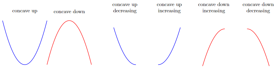
Concave Up and Concave Down

A function is concave up if it “opens” upward. A function is concave down if it “opens” downward.

A point \(x=c\) is called an inflection point of \(f(x)\) if the graph of \(f(x)\) is continious and its concavity changes at \(x=c\).

Suppose the graph of \(f(x)\) is concave up as given below. Draw tangent lines across the inputs of \(f(x)\).

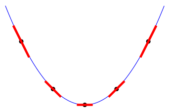
Note that as the value of \(a\) increases, the slope of the tangent line of \(f(x)\) at \(x=a\) also increases (from negative, to zero, to positive).
This implies that if the graph of \(f\,'(x)\) is increasing, then the graph of \(f(x)\) is concave up.
From the previous subsection about Increasing and Decreasing, if the graph of \(f\,''(x)\) is positive then the graph of \(f\,'(x)\) is increasing.

Apply a similar argument for cases where the graph of \(f(x)\) is concave down, we can summarize that if for all \(x\) in some interval \(I\) we have:

• \(f\,''(x)>0\) then \(f(x)\) is concave up on \(I\).

• \(f\,''(x)<0\) then \(f(x)\) is concave down on \(I\).

Note that if \(f\,''(x)=0\) then we cannot guarantee the shape of the graph of \(f(x)\).
\(f\,''(x)=0\) only means the graph of \(f'(x)\) is flat, and many different cases that can cause this. Can you think of these cases?

Below is an example code that asks the user for the function \(f(x)\) and the interval \(I=(a,b)\).
It will plot the graph of \(f(x)\) and \(f\,''(x)\) on \((a,b)\), list all the inflection points, and highlight the area on which \(f(x)\) concave up (or concave down) with green (or red).

Show code cell source Hide code cell source

import matplotlib.pyplot as plt
import numpy as np

def plot_concavity():
    # Prompt the user for the function and interval
    function_input = input("Enter the function f(x): ")
    interval_a = float(input("Enter the left endpoint of the interval (a): "))
    interval_b = float(input("Enter the right endpoint of the interval (b): "))

    # Define the function using numpy
    x = np.linspace(interval_a, interval_b, 1000)
    f = eval("lambda x: " + function_input)

    # Compute the second derivative of f(x)
    f_double_prime = np.gradient(np.gradient(f(x), x), x)

    # Plot the function and concavity
    fig, ax = plt.subplots(figsize=(8, 6))
    ax.plot(x, f(x), label='f(x)', linewidth=1.5)
    ax.plot(x, f_double_prime, label="f''(x)", linewidth=1.5, alpha=0.7)

    # Identify the intervals of concavity
    concave_up_intervals = []
    concave_down_intervals = []

    for i in range(len(x) - 1):
        if f_double_prime[i] > 0:
            concave_up_intervals.append((x[i], x[i + 1]))
        elif f_double_prime[i] < 0:
            concave_down_intervals.append((x[i], x[i + 1]))

    # Add vertical lines for concavity intervals
    for interval in concave_up_intervals:
        ax.axvline(interval[0], color='green', linestyle='--', alpha=0.15, linewidth=0.5)
        ax.axvline(interval[1], color='green', linestyle='--', alpha=0.15, linewidth=0.5)

    for interval in concave_down_intervals:
        ax.axvline(interval[0], color='red', linestyle='--', alpha=0.15, linewidth=0.5)
        ax.axvline(interval[1], color='red', linestyle='--', alpha=0.15, linewidth=0.5)

    # Find the inflection points
    inflection_points = []

    for i in range(1, len(x) - 1):
        if (f_double_prime[i] > 0 and f_double_prime[i + 1] < 0) or (f_double_prime[i] < 0 and f_double_prime[i + 1] > 0):
            inflection_points.append((x[i], f(x[i])))

    # Add points for inflection points
    for point in inflection_points:
        ax.scatter(point[0], point[1], color='blue')

    # Add x-axis and y-axis
    ax.axhline(0, color='black', linewidth=0.5)  # Horizontal line for x-axis
    ax.axvline(0, color='black', linewidth=0.5)  # Vertical line for y-axis

    # Set plot labels and legend
    ax.set_xlabel('x')
    ax.set_ylabel('y')
    ax.set_title('Concavity of f(x)')
    ax.legend()

    # Show the plot
    plt.show()

    # Print the inflection points
    print("Inflection Points:")
    for point in inflection_points:
        print(f'({point[0]:.3f}, {point[1]:.3f})')

# Run the function to plot the concavity
plot_concavity()

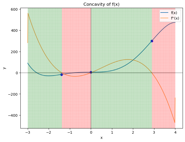
Inflection Points:
(-1.388, -16.236)
(-0.001, 5.000)
(2.886, 298.696)

8.4.4. Extrema

Many applications of Calculus revolve around maximizing or minimizing values of a function.
While visualizing the extrema can be done by analyzing the graph of the function, it might be computationally cheaper to find the extrema using derivatives.

Definition

Relative Extrema

• \(f(x)\) has a relative (or local) maximum at \(x=a\) if \(f(x)>f(a)\) for every \(x\) in some open interval around \(x=a\) (in the “local” neighborhood of \(x=a\)).

• \(f(x)\) has a relative (or local) minimum at \(x=a\) if \(f(x)<f(a)\) for every \(x\) in some open interval around \(x=a\) (in the “local” neighborhood of \(x=a\)).

Relative extrema cannot happen at the endpoints of the domain (since the open interval around \(x=a\) should include some value both to the left and right of \(x=a\)).

Absolute Extrema

• \(f(x)\) has a absolute (or global) maximum at \(x=a\) if \(f(x)\leq f(a)\) for every \(x\) in the domain of \(f\).

• \(f(x)\) has a absolute (or global) minimum at \(x=a\) if \(f(x)\geq f(a)\) for every \(x\) in the domain of \(f\).

Extreme Value Theorem

Theorem: Suppose that \(f(x)\) is continuous on the interval \([a,b]\) then there are two numbers \(c,d\) where \(a\leq c\) and \(d\leq b\) such that \(f(c)\) is an absolute maximum for \(f\) and \(f(d)\) is an absolute minimum of \(f\).

Note that this theorem doesn’t provide the information on where the absolute extrema are, or whether they will occur more than once. It only says that absolute extrema exists somewhere in the interval.

On the other hand, since relative extrema cannot occur at the endpoints, the existence of relative extrema is not guaranteed.

One easy example is the constant function \(f(x)=k\) for some real number \(k\).
This function has no relative extrema in any interval, but the absolute max and absolute min are both \(k\) (that occurs infinitely many times at every point in the domain).

Finding Extrema

A critical number of a function \(f(x)\) is \(x=c\) where \(f(c)\) exists, but either \(f\,'(c)=0\) or \(f\,'(c)\) does not exist. The point \((c,f(c))\) is called a critical point.

• \(f\,'(c)=0\) means the tangent line of \(f(x)\) at \(x=c\) has slope \(0\), meaning it is a horizontal tangent line.
  This can happen on the relative max, relative min, or an inflection point(concave up or down).

• \(f\,'(c)\) does not exist, which means there is no tangent line, or a tangent line exists but is vertical (has an undefined slope).
  This can happen at a corner/cusp when the function is not continuous, or at an inflection point.

Using critical numbers, we have the First Derivative Test:

First Derivative Test
Suppose that \(x=c\) is a critical point of \(f(x)\), then:

• If \(f\,'(x)\) change sign from \(+\) to \(-\) at \(x=c\), then \(f(x)\) has a relative maximum at \(x=c\).

• If \(f\,'(x)\) change sign from \(-\) to \(+\) at \(x=c\), then \(f(x)\) has a relative minimum at \(x=c\).

• If \(f\,'(x)\) doesn’t change sign at \(x=c\), then \(f(x)\) has neither a relative maximum nor a relative minimum at \(x=c\).
  

Going further to the second derivative, recall the relation between the second derivative \(f\,''(x)\) and the shape of graph \(f(x)\).
Note that a concave up graph has a lowest point while a concave down graph has a highest point, which we will use for the Second Derivative Test:

Second Derivative Test
Suppose that \(x=c\) is a critical point of \(f(x)\) such that \(f\,'(c)=0\) and that \(f\,''(x)\) is continuous in the local neighborhood around \(x=c\), then:

• If \(f\,''(x)<0\), then \(f(x)\) has a relative maximum at \(x=c\).

• If \(f\,''(x)>0\), then \(f(x)\) has a relative minimum at \(x=c\).

• If \(f\,''(x)=0\), then at \(x=c\) the function \(f(x)\) can have a relative maximum, relative minimum, or neither.

Summarizing, below are the steps to find extrema given a continuous function \(f(x)\) on the interval \([a,b]\):

• Find the critical points

• Do the first or second derivative test to get the relative extrema

• Evaluate and compare the values of \(f(x)\) at the critical points and the endpoints to get the absolute extrema

It is left to motivated students to do these steps manually.
Below is the example code that asks the user to give \(f(x)\) and the endpoints of closed interval \([a,b]\). Code will return the list of absolute and relative extrema.

Show code cell source Hide code cell source

def find_extrema():
    # Prompt the user for the function and interval
    function_input = input("Enter the function f(x): ")
    interval_a = float(input("Enter the left endpoint of the interval (a): "))
    interval_b = float(input("Enter the right endpoint of the interval (b): "))

    # Convert the function string to a SymPy expression
    x = sp.Symbol('x')
    f = sp.sympify(function_input)

    # Evaluate the function at critical points and exclude endpoints
    critical_points = sp.solve(sp.diff(f, x), x)
    critical_points = [point for point in critical_points if interval_a < point < interval_b]

    # Evaluate the function at the endpoints
    endpoints = [interval_a, interval_b]
    extrema_coordinates = [(round(point, 3), round(f.subs(x, point), 3)) for point in critical_points]

    # Find the absolute maximum and minimum
    extrema_coordinates.extend([(interval_a, round(f.subs(x, interval_a), 3)), (interval_b, round(f.subs(x, interval_b), 3))])
    absolute_max = max(extrema_coordinates, key=lambda coord: coord[1])
    absolute_min = min(extrema_coordinates, key=lambda coord: coord[1])

    # Find the relative maxima and minima
    relative_maxima = []
    relative_minima = []

    for point in critical_points:
        second_derivative = sp.diff(f, x, 2).subs(x, point)
        if second_derivative < 0:
            relative_maxima.append((point, round(f.subs(x, point), 3)))
        elif second_derivative > 0:
            relative_minima.append((point, round(f.subs(x, point), 3)))

    # Print the extrema coordinates
    print("Relative Maxima:")
    if len(relative_maxima) > 0:
        for coordinate in relative_maxima:
            print(coordinate)
    else:
        print("none")

    print("Relative Minima:")
    if len(relative_minima) > 0:
        for coordinate in relative_minima:
            print(coordinate)
    else:
        print("none")

    print("Absolute Maximum:")
    print(absolute_max)

    print("Absolute Minimum:")
    print(absolute_min)

# Run the function to find the extrema
find_extrema()

Relative Maxima:
(4.00000000000000, 474.333)
Relative Minima:
(-2.00000000000000, -29.667)
Absolute Maximum:
(-4.0, 815.667)
Absolute Minimum:
(-2.00000000000000, -29.667)

8.4.5. The Mean Value Theorem

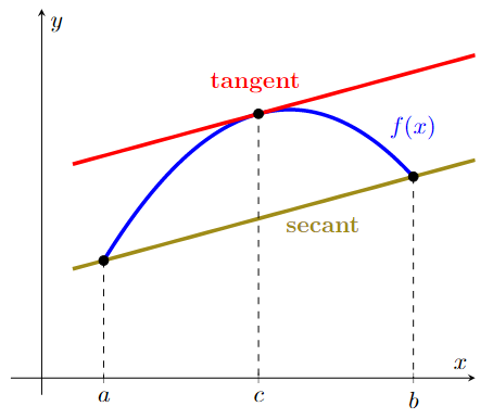
Also called the Lagrange Theorem, the Mean Value Theorem (MVT) stated that:
If \(f\) is a continuous function on the closed interval \([a,b]\) and differentiable on the open interval \((a,b)\), then there is a point \(c\) in \((a,b)\) such that the tangent at \(c\) is parallel to the secant line throught the endpoints \((a,f(a))\) and \((b,f(b))\), that is, \(f\,'(c)=\dfrac{f(b)-f(a)}{b-a}\), or, \(f(b)-f(a)=f\,'(c)(b-a)\).

Note that MVT doesn’t give what \(c\) is. It only guarantees the existence of at least one of such \(c\). Finding the \(c\) can be done manually or using code.

Example

Determine the number(s) \(c\) which satisfies the conclusion of the MVT for the function \(f(x)=4x-x^2\) on \([0.5,3]\).

The derivative of \(f(x)\) is \(f\,'(x)=4-2x\). From the conclusion of the MVT we have \(4-2c=f\,'(c) =\dfrac{f(3)-f(0.5)}{3-0.5}=\dfrac{1.25}{2.5}=0.5\), giving \(c=1.75\) as the only such \(c\).

Below is the code that prompts the user to provide \(f(x)\) and the interval endpoints \(a\) and \(b\), then returns the value(s) of \(c\) satisfying the conclusion of MVT.

Show code cell source Hide code cell source

# Prompt the user for the function f(x)
equation = input("Enter the function f(x): ")

# Define the variable x
x = sp.Symbol('x')

# Create a SymPy expression for f(x)
f_expr = sp.sympify(equation)

# Prompt the user for the values of a and b
a = float(input("Enter the value of a: "))
b = float(input("Enter the value of b: "))

# Compute the derivative of f(x)
f_prime_expr = sp.diff(f_expr, x)

# Compute the right-hand side of the equation
rhs = (f_expr.subs(x, b) - f_expr.subs(x, a)) / (b - a)

# Find all values of c that satisfy f'(c) = (f(b) - f(a))/(b - a)
solutions = sp.solve(sp.Eq(f_prime_expr, rhs), x)

# Print the values of c
print("Values of c that satisfy the conclusion of MVT:")
for c in solutions:
    print(f"c = {c.evalf()}")  # Evaluate the symbolic solution

Values of c that satisfy the conclusion of MVT:
c = 1.75000000000000

Example

Given \(f(x)\) a continuous and differentiable function on \([2,10]\). It is known that \(f(2)=-5\) and \(f\,'(x)\leq 6\). What is the largest possible value for \(f(10)\)?
From the conclusion of MVT, we have \(f(10)-f(2)=f\,'(c)(10-2)\), so \(f(10)=f(2)+f\,'(c)(10-2)=-5+8f\,'(c)\).
Since \(f\,'(x)\leq 6\) then \(f\,'(c)\leq 6\). Thus \(f(10)=-5+8f\,'(c)\leq -5+8(6)=43\). Thus, the largest possible value for \(f(10)\) is 43.

8.4.6. Linearization

Recall that \(f\,'(a)\) is the slope of the tangent line of \(f(x)\) at \(x=a\). Conversely, given a function \(f(x)\), the equation of the tangent line that touch \(f(x)\) at \(x=a\) using derivative \(f\,'(a)\) is given by \(L(x)=f(a)+f\,'(a)(x-a)\).

Look at the graph of a function \(f(x)\) with its tangent line at \(x=a\) below:

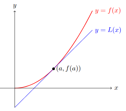
Note that the values of \(f(x)\) and \(L(x)\) get closer and closer as \(x\to a\), so we can use \(L(x)\) to approximate the value of \(f(x)\) near \(x=a\).
Due to this, this tangent line \(L(x)\) is often called the linear approximation or linearization of \(f(x)\) at \(x=a\).

Example

Find the linearization for \(f(x)=\sqrt[3]{x}\) at \(x=27\), and use it to approximate \(\sqrt[3]{27.137}\) and \(\sqrt[3]{8}\).
Now \(f(27)=\sqrt[3]{27}=3\) and using power rule get \(f\,'(x)=\dfrac{1}{3}x^{2/3}=\dfrac{1}{3\sqrt[3]{2}}\) so \(f\,'(x)=\dfrac{1}{27}\).
The linearization is then \(L(x)=3+\dfrac{1}{27}(x-27)\).

Thus \(\sqrt[3]{27.137}\approx L(27.137) =3+\dfrac{1}{27}(0.137) = 3.00507\overline{407}\) and \(\sqrt[3]{8}\approx L(8) =3+\dfrac{1}{27}(-19) = 2.\overline{296}\).

Comparing with the actual value \(\sqrt[3]{27.137}\approx 3.005065516\ldots\) and \(\sqrt[3]{8}=2\), see that the approximation for \(\sqrt[3]{27.137}\) is much more accurate than the approximation for \(\sqrt[3]{8}\).
This makes sense since \(8\) is much further from \(27\) compared to \(27.137\) and hence the distance between the curve of \(f(x)\) and the tangent line \(L(x)\) is much further as well.

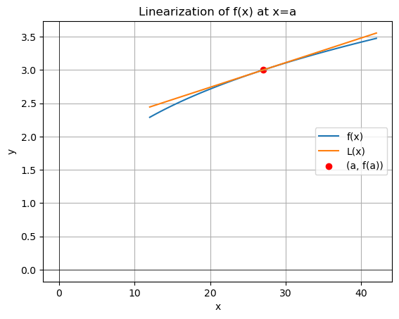
Below is the code that prompts the user to give the function \(f(x)\) and the point \(x=a\). The code return equation \(L(x)\) at \(x=a\) as well as their plots.

Show code cell source Hide code cell source

# Prompt user for the function f(x) and a value of x=a
equation = input("Enter the function f(x): ")
a = float(input("Enter the value of x (a): "))

# Create a symbolic expression for the given equation
x = sp.symbols('x')
f_expr = sp.sympify(equation)
f = sp.lambdify(x, f_expr)

# Calculate the derivative of f(x) at x=a
f_prime = sp.diff(f_expr, x).subs(x, a)

# Calculate the linearization L(x) at x=a
L_expr = f(a) + f_prime * (x - a)
L = sp.lambdify(x, L_expr)

# Generate x values from a-15 to a+15
x_vals = np.linspace(a - 15, a + 15, 100)

#Print the linearization L(x)
print("Equation of L(x):", sp.latex(L_expr))

# Plot f(x), L(x), and the point (a, f(a))
plt.plot(x_vals, f(x_vals), label="f(x)")
plt.plot(x_vals, L(x_vals), label="L(x)")
plt.scatter(a, f(a), color="red", label="(a, f(a))")
plt.xlabel("x")
plt.ylabel("y")
plt.title("Linearization of f(x) at x=a")
plt.legend()
plt.grid(True)
plt.axhline(0, color="black", linewidth=0.5)
plt.axvline(0, color="black", linewidth=0.5)
plt.show()

Equation of L(x): 0.037037037037037 x + 2.0

8.4.7. Implicit Differentiation

So far we have discussed derivatives of functions of the form \(y=f(x)\). However, there are cases where the equations relating \(y\) and \(x\) either cannot be written explicitly as \(y=f(x)\), or writing it as \(y=f(x)\) results in some issues in finding the derivative. In these cases, we can use implicit differentiation.

Example

• Writing the equation \(e^{x+2y}=\ln\left(xy^2\right)+x^2\) in the form \(y=f(x)\) is challenging at best.

• Writing the equation \(x^2+y^2=4\) in the form \(y=f(x)\) gives \(y=\pm\sqrt{4-x^2}\), but then how to deal with the \(\pm\) for the derivative if we only want to write the derivative as a single function?

With implicit differentiation, we can treat the variable \(y\) as \(y(x)\) and utilize Chain Rule as we derive both sides and obtain the derivative as a single function that likely will have both \(x\) and \(y\). Below is the example for the equation \(x^2+y^2=4\):

\[\begin{split} \begin{align} \dfrac{d}{dx}\left(x^2+\left[y(x)\right]^2\right) &=\dfrac{d}{dx}[4]\\ 2x+2\cdot y(x)\cdot y\,'(x) &=0 \\ 2x+2yy\,'&=0\\ 2yy\,'&=-2x\\ y\,'&=-\dfrac{x}{y} \end{align} \end{split}\]

While Python does not have built-in functionality specifically dedicated to implicit differentiation, we can leverage SymPy to perform implicit differentiation. Depending on the complexity of the equation, further algebraic manipulation or specific handling may be required. Below is a code example, prompting the user to input the equation. For \(x^2+y^2=4\), first rewrite into \(x^2+y^2-4=0\) and input the nonzero side as the equation:

Show code cell source Hide code cell source

# Prompt the user to input the equation
equation_str = input("Enter the equation: ")

# Define the variables
x, y = sp.symbols('x y')

# Convert the equation string to a SymPy expression
equation = sp.sympify(equation_str)

# Differentiate implicitly
diff_eq = sp.diff(equation, x)  # Differentiate with respect to x
diff_eq_y = sp.diff(equation, y)  # Differentiate with respect to y

# Solve for dy/dx using the chain rule
dy_dx = -diff_eq / diff_eq_y

# Simplify the result
dy_dx_simplified = sp.simplify(dy_dx)

# Print the result
print("The derivative dy/dx is:", dy_dx_simplified)

The derivative dy/dx is: -x/y

8.4.8. Exercises

Exercises

1. (Section 4.1) Find the derivative of the following functions using the limit definition of the derivative.

   • \(f(x)=3x^2-12x+32\)

   • \(g(x)=\dfrac{x}{x+2}\)

   • \(h(x)=\sqrt{4x^2-6}\)

2. (Section 4.1) Prove \(\left[f \pm g\right]' = f' \pm g'\) using the limit definition of the derivative.

3. (Section 4.2) Find the derivative of the following functions using the appropriate properties, formulas, and/or rules. Compare the result by using code.

   • \(f(x)=3x^2-12x+32\)

   • \(g(x)=\dfrac{x}{x+2}\)

   • \(h(x)=\sqrt{4x^2-6}\)

   • \(z(x)=x^5\sin\left(3x^4+1\right)+\ln\left(20^x-e^{5x}\right)\)

4. (Section 4.2) Find the derivative of the following function using both Product and Quotient Rule, and verify that they gives the same answer.

   • \(a(x)=\dfrac{\sin(x)}{x}\)

   • \(b(x)=\dfrac{\cos(x)}{2-x^9}\)

   • \(c(x)=\dfrac{\sin\left(3+4^x\right)}{2-x^9}\)

5. (Section 4.2) Use Quotient Rule and the Basic Derivative formulas for \(\sin(x)\) and \(\cos(x)\), to find the derivative of \(\tan(x),\cot(x),\sec(x),\) and \(\csc(x)\).

6. (Section 4.3) Find the interval(s) in which the following functions is increasing, decreasing, concave up, concave down.

   • \(a(x)=2x^3+3x^2-12x+4\) on \([-4,3]\)

   • \(b(x)=3x+\sin(4x)\) on \([0,1]\)

7. (Section 4.4) Find the absolute and relative extrema of the following functions:

   • \(a(x)=2x^3+3x^2-12x+4\) on \([-4,3]\)

   • \(b(x)=3x+\sin(4x)\) on \([0,1]\)

8. (Section 4.5) Use the MVT to do the following problems:

   • Determine all the number(s) \(c\) which satisty the conclusion of the MVT for the function \(f(x)=4x^3-8x^2+7x-2\) on \([-3,5]\)

   • Given \(f(x)\) a continuous and differentiable function on \([-3,2]\). It is known that \(f(-3)=5\) and \(f\,'(x)\geq 7\). What is the smallest possible value for \(f(2)\)?

9. (Section 4.6) Find the linearization for each given function at each given points, and plot the graph together with their linearization.
   For each, also use the linearlization to approximate the value at the given nearby point, then calculate the error of the approximation.

   • \(f(x)=\sqrt[4]{x}\) at \(x=16\), use to approximate \(\sqrt[4]{16.7}\)

   • \(g(x)=\sin(x)\) at \(x=\dfrac{\pi}{4}\), use to approximate \(\sin\left(\dfrac{3\pi}{11}\right)\)

10. (Section 4.7) Use implicit differentiation to find \(y\,'\) for each of the following:

    • \(5x+x^4y^3=7y^3-2\)

    • \(3x^2\tan(y)=x-y^5\sec{x}\)

    • \(e^{x+2y}=\ln\left(xy^2\right)+x^2\)