11.7. Solutions to Exercises

11.7.1. Section 2 Solutions

1. List the type and order of each of the following differential equations. For each ordinary differential equation, determine if it is linear or nonlinear.

   • \(\dfrac{dQ}{dt} = \dfrac{tP}{100}\)

     • Linear first-order ordinary differential equation

   • \(\frac{\partial^2 v}{\partial t^2} + \frac{\partial^2 v}{\partial w^2} = 5\)

     • Second-order partial differential equation

   • \(2\dfrac{d^2q}{dt^2} + \cos(t) \dfrac{dq}{dt} = E(t)\)

     • Linear second-order ordinary differential equation

2. Show that \(f(x) = \sin(x)+\cos(x)+x^2-2\) is a solution for all \(x\) to \(y''+y = x^2\).

import sympy as sym

x = sym.Symbol('x')
#Define f(x)
f = sym.sin(x)+sym.cos(x)+x**2-2
print('This is the function f(x):', f)

#Define f'(x)
dfdx = sym.diff(f)
print('This is the derivative of f(x):', dfdx)

#Define f''(x)
dfdxx = sym.diff(dfdx)
print('This is the second derivative of f(x):', dfdxx)

#See if f(x) is a solution to the differential equation. If it outputs True, f(x) is a solution.
dfdxx+f == x**2

This is the function f(x): x**2 + sin(x) + cos(x) - 2
This is the derivative of f(x): 2*x - sin(x) + cos(x)
This is the second derivative of f(x): -sin(x) - cos(x) + 2

True

Section 3 Solutions

1. Determine if the following first-order differential equations are linear, separable, both, or neither.

   • \(\frac{dy}{dx} = y + x\)

     • Linear, but not separable

   • \(\sqrt{y} + 2\frac{dy}{dx} = e^{x}\)

     • Neither- the square root makes this non-linear

   • \(\sqrt{y}\frac{dy}{dx} = e^{x}\)

     • Separable, but not linear

   • \(\frac{dy}{dx} = x+5\)

     • Both linear and separable

2. Find the explicit solution to the differential equation \(y'(x) = y+5\).

   \[\dfrac{dy}{y+5} = dx \]
   \[\ln|y+5| = x + C \]
   \[y+5 = e^{x + C} \]

   • Solution: \(y(x) = C_1e^x-5\)

   Note: The reason that the solution can be written as such is because \( e^{x + C} \) can be rewritten as \( e^{x}e^{C} \); since \(C\) itself is already an arbitrary constant, \( e^{C} \) can simply become the new arbitrary constant, which is then named \(C_1\). Sometimes, teachers will just name the new constant \(C\) instead of \(C_1\) for simplicity, although \(C_1\) is technically more accurate, as it is a new constant. This simplification is common and helps keep expressions concise. \( \)

3. Find the explicit solution to the differential equation \(W'(s) = s+sW^2\).

   \[\dfrac{dW}{1+W^2} = s ds \]
   \[\arctan(W) = \dfrac{s^2}{2} + C \]

   • Solution: \(W(s) = \tan\left(\dfrac{s^2}{2}+C \right)\)

4. Find the explicit solution to the initial value problem \(y'(t) = ty\) where \(y(0)=3\).

   \[\dfrac{dy}{y} = t dt \]
   \[\ln|y| = \dfrac{t^2}{2} + C \]
   \[y = Ce^{\dfrac{t^2}{2}} \]
   \[3 = Ce^{0}\]
   \[C=3\]

   • Solution: \(y(t) = 3e^{\dfrac{t^2}{2}}\)

5. Find the explicit solution to the initial value problem \(x'(t) = x\sin(t)\) where \(x(0)=1\).

   \[\dfrac{dx}{x} = \sin(t) dt \]
   \[\ln|x| = -\cos(t) + C \]
   \[x = Ce^{-\cos(t)} \]
   \[1 = Ce^{-1}\]
   \[C=e\]

   • Solution: \(x(t) = e*e^{-\cos(t)}\)

6. Show that if a first order differential equation is both linear and homogeneous, then it is also separable.

   • Let \(a_1(t)\dfrac{dx}{dt} + a_0(t)x(t) = 0\) be an arbitary homogeneous linear first order differential equation. This means that \(\dfrac{dx}{dt} = \dfrac{-a_0(t)x(t)}{a_1(t)}\). Dividing both sides by \(x(t)\) allows us to separate the variables in the following way \(\dfrac{1}{x(t)}\dfrac{dx}{dt} = \dfrac{-a_0(t)}{a_1(t)}\).

7. Find the solution to the differential equation \(\frac{dP}{dt} = \frac{2P}{t} + t^2\sec^2(t)\). Note: This differential equation is not in standard form so we need to first put it in standard form prior to applying the method of the integrating factor.

\[\frac{dP}{dt} - \frac{2P}{t} = t^2\sec^2(t)\]

\[\mu(t) = e^{\int \dfrac{-2}{t} dt} = e^{-2\ln(t)} = t^{-2}\]

\[t^{-2}\frac{dP}{dt} - \frac{2P}{t^3} = \sec^2(t)\]

\[\frac{d}{dt}(t^{-2}\cdot P(t)) = t^{-2}\frac{dP}{dt} - \frac{2P}{t^3}\]

\[\frac{d}{dt}(t^{-2}\cdot P(t)) = \sec^2(t)\]

\[\displaystyle{\int \frac{d}{dt}(t^{-2}\cdot P(t)) dt = \int \sec^2(t) dt}\]

\[t^{-2}\cdot P(t) = \tan(t)+C\]

• Solution: \(P(t) = t^2(\tan(t)+C)\)

8. Find the solution to the initial value problem \(xy' + y = \sin(x)\), where \(y(\pi)=0\). Note: This differential equation is not in standard form, so we need to first put it in standard form prior to applying the method of the integrating factor.

\[\frac{dy}{dx} + \frac{y}{x} = \dfrac{\sin(x)}{x}\]

\[\mu(t) = e^{\int \dfrac{1}{x} dx} = e^{\ln(x)} = x\]

\[x\dfrac{dy}{dx} + y = \sin(x)\]

\[\frac{d}{dx}(x\cdot y(x)) = x\dfrac{dy}{dx} + y\]

\[\frac{d}{dx}(x\cdot y(x)) = \sin(x)\]

\[\displaystyle{\int \frac{d}{dx}(x\cdot y(x)) dx = \int \sin(x) dx}\]

\[x\cdot y(x) = -\cos(x)+C\]

\[y(x) = \dfrac{-\cos(x)+C}{x}\]

\[0 = \dfrac{-\cos(\pi)+C}{\pi}\]

\[C=-1\]

• Solution: \(y(x) = \dfrac{-\cos(x)-1}{x}\)

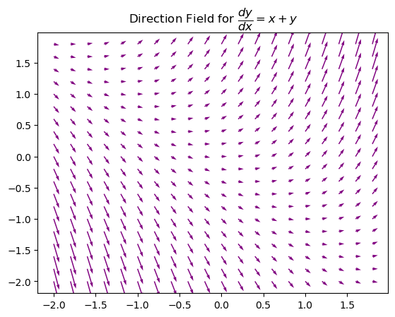
9. Plot a direction field for \(y'(x) = y+x\).

import numpy as np
import matplotlib.pyplot as plt

#Take some time to play around with the various parameters and see how it impacts the slope-field that is produced.
nx, ny = .2, .2
x = np.arange(-2,2,nx)
y = np.arange(-2,2,ny)

#Create a rectangular grid with points
X,Y = np.meshgrid(x,y)

#Define the functions
dy = X+Y
dx = np.ones(dy.shape)

#Plot
plt.quiver(X,Y,dx,dy,color='purple')
plt.title('Direction Field for $ \dfrac{dy}{dx} = x+y $')
plt.show()

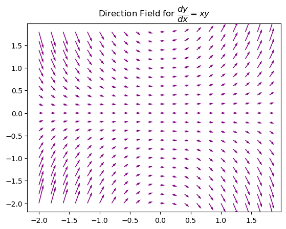
10. Plot a direction field for \(y'(x) = xy\).

import numpy as np
import matplotlib.pyplot as plt

#Take some time to play around with the various parameters and see how it impacts the slope-field that is produced.
nx, ny = .2, .2
x = np.arange(-2,2,nx)
y = np.arange(-2,2,ny)

#Create a rectangular grid with points
X,Y = np.meshgrid(x,y)

#Define the functions
dy = X*Y
dx = np.ones(dy.shape)

#Plot
plt.quiver(X,Y,dx,dy,color='purple')
plt.title('Direction Field for $ \dfrac{dy}{dx} = xy $')
plt.show()

11. Find the equilibrium solutions of \(y'(x) = \sin(y)\).

    • \(\sin(y)=0\) when \(y=\dfrac{\pi k}{2}\) where \(k\) is an even integer.

12. Draw a phase line and determine where a solution of the differential equation \(\frac{dT}{dt} = (T+1)T(T-3)^2\) is increasing and decreasing. Then classify the stability of each equilibrium point.

import numpy as np
import matplotlib.pyplot as plt

# Function for the autonomous differential equation
def f(T):
    return (T+1) * T * (T - 3)**2

# Identify the critical points (where dT/dt = 0)
critical_points = [-1, 0, 3]

# Create the figure and axis
fig, ax = plt.subplots()

# Plot the phase line at x = 0 with markers at the critical points
for point in critical_points:
    if f(point - 0.01) > 0 > f(point + 0.01):
        ax.plot(0, point, 'go')  # Stable points in green
    elif f(point - 0.01) < 0 < f(point + 0.01):
        ax.plot(0, point, 'ro')  # Unstable points in red
    else:
        ax.plot(0, point, 'yo') # Semi-stable point in yellow
        
# Draw arrows indicating direction of movement
arrow_properties = dict(facecolor='black', width=0.075, head_width=.3, head_length=.3)  # Decrease head_width to make arrows skinnier

check_points = [-1.5, -0.1, 1.5, 3.5]

# Check below the lowest critical point separately
if f(check_points[0]) > 0:
    ax.arrow(0, (check_points[0] - 2)/1.8, 0, 0.3, **arrow_properties)  # Pointing up if derivative is positive
else:
    ax.arrow(0, (check_points[0] - 2)/1.8, 0, -0.3, **arrow_properties)  # Pointing down if derivative is negative

for i in range(len(critical_points) - 1):
    if f(check_points[i+1]) > 0:
        ax.arrow(0, (critical_points[i] + critical_points[i+1])/2.2, 0, 0.3, **arrow_properties)  # Pointing up if derivative is positive
    else:
        ax.arrow(0, (critical_points[i] + critical_points[i+1])/2.2, 0, -0.3, **arrow_properties)  # Pointing down if derivative is negative

# Check above the highest critical point separately
if f(check_points[-1]) > 0:
    ax.arrow(0, (critical_points[-1] + 3)/1.8, 0, 0.3, **arrow_properties)  # Pointing up if derivative is positive
else:
    ax.arrow(0, (critical_points[-1] + 3)/1.8, 0, -0.3, **arrow_properties)  # Pointing down if derivative is negative

# Set the y-axis limits
plt.ylim(-2.1, 4.1)
# Set the x-axis limits
plt.xlim(-0.5, 0.5)

# Label the y-axis
plt.ylabel('T')

# Title of the plot
plt.title('Phase Line Plot')

# Remove the x-axis
plt.gca().axes.get_xaxis().set_visible(False)

# Show the plot
plt.show()

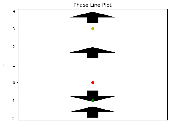
Using the above diagram, \(-1\) is a stable equilibrium, \(0\) is an unstable equilibrium, and \(3\) is a semi-stable equilibrium.

Section 4 Solutions

1. Find all solutions to \(x''+x'-6x=0\). Suppose \(x(t)=e^{kt}\) is a solution. This means it satisfies our differential equation. Since \(x'(t) = ke^{kt}\) and \(x''(t) = k^2e^{kt}\), we know

\(x'' +x' -6x = k^2e^{kt} +ke^{kt}-6e^{kt} = e^{kt}(k^2+k-6)=0\).

Since \(e^{kt} \neq 0\), we know that \(k^2+k-6=0\) when \(e^{kt}\) is a solution. Thus, \(k^2+k-6=0\) is the characteristic equation of this differential equation. Solving the characteristic equation gives \(k^2+k-6=0=(k+3)(k-2)=0\). Thus, \(k=-3\) and \(k=2\) are the solutions.

This means that \(\{e^{-3t},e^{2t}\}\) is the fundamental set of solutions and thus, the general solution \(x(t)= c_1e^{-3t} + c_2e^{2t}\) does capture all solutions of this differential equation.

2. Use your answer to 1 to find the general solution to the differential equation \(x''+x'-6x=\sin(3t)\).

From Problem 1, we know that the solution to the associated homogeneous equation is \(x_h(t)= c_1e^{-3t} + c_2e^{2t}\).

We now need to find the particular solution. Using the chart, we know that \(x_p(t) = A\sin(3t)+B\cos(3t)\). Furthermore, \(x_p'(t) = 3A\cos(3t)-3B\sin(3t)\) and \(x_p''(t) = -9A\sin(3t)-9B\cos(3t) = -9x_p(t)\). Plugging this into the differential equation gives

\[x_p''(t)+ x_p'(t)-6x_p(t) = \sin(3t) \]

\[-9x_p(t)+ x_p'(t)-6x_p(t) = \sin(3t) \]

\[x_p'(t)-15x_p(t) = \sin(3t) \]

\[3A\cos(3t)-3B\sin(3t)-15(A\sin(3t)+B\cos(3t)) = \sin(3t) \]

\[(3A-15B)\cos(3t)+(-15A-3B)\sin(3t) = \sin(3t) \]

Thus we know that \(3A-15B=0\) and \(-15A-3B=1\). This gives that \(A = \dfrac{-5}{78}\) and \(B = \dfrac{-1}{78}\). Thus \(x_p(t) = \dfrac{-5}{78}\sin(3t)+\dfrac{-1}{78}\cos(3t)\). So the general solution is

\[x(t) = x_h(t) + x_p(t) = c_1e^{-3t} + c_2e^{2t} + \dfrac{-5}{78}\sin(3t)+\dfrac{-1}{78}\cos(3t).\]

3. Use your answer to 1 to find the general solution to the differential equation \(x''+x'-6x=5e^{4t}\).

From Problem 1, we know that the solution to the associated homogeneous equation is \(x_h(t)= c_1e^{-3t} + c_2e^{2t}\).

We now need to find the particular solution. Using the chart, we know that \(x_p(t) = Ae^{4t}\). Furthermore, \(x_p'(t) = 4Ae^{4t}\) and \(x_p''(t) = 16Ae^{4t}\). Plugging this into the differential equation gives

\[x_p''(t)+ x_p'(t)-6x_p(t) = 5e^{4t} \]

\[16Ae^{4t}+ 4Ae^{4t}-6Ae^{4t} = 5e^{4t} \]

\[14Ae^{4t} = 5e^{4t} \]

Thus we know \(A = \dfrac{5}{14}\). Thus \(x_p(t) = \dfrac{5}{14}e^{4t}\). So the general solution is

\[x(t) = x_h(t) + x_p(t) = c_1e^{-3t} + c_2e^{2t} + \dfrac{5}{14}e^{4t}.\]

4. Use your answer to 1 to find the general solution to the differential equation \(x''+x'-6x=5e^{2t}\). Hint: Think about why changing the exponent from \(4t\) to \(2t\) adds an extra step to the problem.

From Problem 1, we know that the solution to the associated homogeneous equation is \(x_h(t)= c_1e^{-3t} + c_2e^{2t}\).

We now need to find the particular solution. Using the chart, we know that \(x_p(t) = Ae^{2t}\). But, this isn’t linearly independent from \(x_h(t)\) so we must multiple our particular solution by \(t\). Therefore, our updated \(x_p(t) = Ate^{2t}\). Furthermore, \(x_p'(t) = Ae^{2t}+2tAe^{2t}\) and \(x_p''(t) = 4Ae^{2t}+4Ate^{2t}\). Plugging this into the differential equation gives

\[x_p''(t)+ x_p'(t)-6x_p(t) = 5e^{2t} \]

\[4Ae^{2t}+4Ate^{2t}+ Ae^{2t}+2tAe^{2t}-6Ate^{2t} = 5e^{2t} \]

\[5Ae^{2t} = 5e^{2t} \]

Thus we know \(A = 1\). Thus \(x_p(t) = te^{2t}\). So the general solution is

\[x(t) = x_h(t) + x_p(t) = c_1e^{-3t} + c_2e^{2t} + te^{2t}.\]

5. Use your answer to 2 and 3 to find the general solution of the differential equation \(x''+x'-6x = 5e^{4t}+\sin(3t)\). Hint: What does the Superposition Principle tell us?

From Problem 2 and Problem 3, we can read off the general solution. In particular, we know

\[x(t) = c_1e^{-3t} + c_2e^{2t} + \dfrac{5}{14}e^{4t}+ \dfrac{-5}{78}\sin(3t)+\dfrac{-1}{78}\cos(3t).\]

6. Find the form of the particular solution of the following differential equations. Note you do not need to solve for the undetermined coefficients.

   • \(x''-6x'+9x = 3t+10\cos(t)\)

     • \(x_p(t) = At+B+C\cos(t)+D\sin(t)\)

   • \(x''-9x=te^{3t}\)

     • \(x_p(t) = (At+B)Ce^{3t}\), which can be simplified to \(x_p(t) = (Dt + E)e^{3t}\)

   • \(2x''+x'+4x = 3t^2\sin(2t)\)

     • \(x_p(t) = (At^2+Bt+C)(D\cos(2t)+E\sin(2t))\)

Section 5 Solutions

1. Which of the following sets are linearly independent?

• \(\biggl\{\begin{bmatrix} e^{2t} \\ e^{4t} \end{bmatrix}, \begin{bmatrix} e^{2t} \\ e^{7t} \end{bmatrix}\biggr\}\)

  • These are linearly independent because of the second coordinate in each vector.

• \(\biggl\{\begin{bmatrix} \cos(t) \\ -e^{3t} \end{bmatrix}, \begin{bmatrix} -\cos(t) \\ e^{3t} \end{bmatrix}\biggr\}\)

  • These are not linearly independent. Notice that adding the two vectors together produces the zero vector.

• \(\biggl\{v_1(t) = \begin{bmatrix} \sin^2(4t) \\ t \end{bmatrix}, v_2(t)= \begin{bmatrix} \cos^2(4t) \\ 3t \end{bmatrix}, v_3(t) = \begin{bmatrix} 1 \\ 4t \end{bmatrix}\biggr\}\)

  • These are not linearly independent as \(v_1(t)+v_2(t)-v_3(t) =\vec{0}\)

2. Solve the initial-value problem

\[\begin{split} x' = \begin{bmatrix} -3 & 1 & -1 \\ 0 & -3 & 2 \\ 0 & -1 & 0 \end{bmatrix}x, \quad x(0) = \begin{bmatrix} 1 \\ 1 \\ 0 \end{bmatrix}. \end{split}\]

\[\det(A-\lambda I) = 0\]

\[\begin{split}\det\left(\begin{bmatrix} -3-\lambda & 1 & -1 \\ 0 & -3-\lambda & 2 \\ 0 & -1 & -\lambda \end{bmatrix} \right)=0\end{split}\]

\[(-3-\lambda)(\lambda^2+3\lambda+2)=0\]

\[(-3-\lambda)(\lambda+1)(\lambda+2)=0\]

Thus the eigenvalues are \(\lambda=-3\), \(\lambda=-2\), and \(\lambda=-1\).

Now we want to find the eigenvectors associated to each eigenvalue. Let’s start with \(\lambda =-3\).

Setting up the augmented matrix yields

\[\begin{split} \left[ \begin{bmatrix} 0 & 1 & -1 \\ 0 & 0 & 2 \\ 0 & -1 & -3 \\ \end{bmatrix} \left| \, \begin{matrix} 0 \\ 0 \\ 0 \\ \end{matrix} \right. \right] \approx \left[ \begin{bmatrix} 0 & 1 & 0 \\ 0 & 0 & 1 \\ 0 & 0 & 0 \\ \end{bmatrix} \left| \, \begin{matrix} 0 \\ 0 \\ 0 \\ \end{matrix} \right. \right] \end{split}\]

Thus an eigenvector associated to \(\lambda=-3\) is \(\begin{bmatrix} 1 \\ 0 \\ 0 \end{bmatrix}\).

Let’s now consider \(\lambda = -2\).

Setting up the augmented matrix yields

\[\begin{split} \left[ \begin{bmatrix} -1 & 1 & -1 \\ 0 & -1 & 2 \\ 0 & -1 & -2 \\ \end{bmatrix} \left| \, \begin{matrix} 0 \\ 0 \\ 0 \\ \end{matrix} \right. \right] \approx \left[ \begin{bmatrix} 1 & 0 & -1 \\ 0 & 1 & -2 \\ 0 & 0 & 0 \\ \end{bmatrix} \left| \, \begin{matrix} 0 \\ 0 \\ 0 \\ \end{matrix} \right. \right] \end{split}\]

Thus an eigenvector associated to \(\lambda=-2\) is \(\begin{bmatrix} 1 \\ 2 \\ 1 \end{bmatrix}\).

Let’s now consider \(\lambda = -1\).

Setting up the augmented matrix yields

\[\begin{split} \left[ \begin{bmatrix} -2 & 1 & -1 \\ 0 & -2 & 2 \\ 0 & -1 & 1 \\ \end{bmatrix} \left| \, \begin{matrix} 0 \\ 0 \\ 0 \\ \end{matrix} \right. \right] \approx \left[ \begin{bmatrix} -2 & 0 & 0 \\ 0 & 1 & -1 \\ 0 & 0 & 0 \\ \end{bmatrix} \left| \, \begin{matrix} 0 \\ 0 \\ 0 \\ \end{matrix} \right. \right] \end{split}\]

Thus an eigenvector associated to \(\lambda=-1\) is \(\begin{bmatrix} 0 \\ 1 \\ 1 \end{bmatrix}\).

This means the general solution to this system is \(x(t) = c_1\begin{bmatrix} 0 \\ 1 \\ 1 \end{bmatrix}e^{-t} + c_2\begin{bmatrix} 1 \\ 2 \\ 1 \end{bmatrix}e^{-2t} + c_3\begin{bmatrix} 1 \\ 0 \\ 0 \end{bmatrix}e^{-3t}\).

Using the initial condition, we find that

\[\begin{split} \begin{bmatrix} 1 \\ 1 \\ 0 \end{bmatrix} = c_1\begin{bmatrix} 0 \\ 1 \\ 1 \end{bmatrix}e^{-(0)} + c_2\begin{bmatrix} 1 \\ 2 \\ 1 \end{bmatrix}e^{-2(0)} + c_3\begin{bmatrix} 1 \\ 0 \\ 0 \end{bmatrix}e^{-3(0)} \end{split}\]

\[\begin{split} \begin{bmatrix} 1 \\ 1 \\ 0 \end{bmatrix} = c_1\begin{bmatrix} 0 \\ 1 \\ 1 \end{bmatrix} + c_2\begin{bmatrix} 1 \\ 2 \\ 1 \end{bmatrix} + c_3\begin{bmatrix} 1 \\ 0 \\ 0 \end{bmatrix} \end{split}\]

Solving this system for \(c_1\), \(c_2\), and \(c_3\) gives \(c_1=-1\), \(c_2=1\), and \(c_3=0\).

Thus the solution to the initial value problem is

\[\begin{split} x(t) = -\begin{bmatrix} 0 \\ 1 \\ 1 \end{bmatrix}e^{-t} + \begin{bmatrix} 1 \\ 2 \\ 1 \end{bmatrix}e^{-2t}. \end{split}\]

3. Solve the initial-value problem

\[\begin{split} x' = \begin{bmatrix} 4 & -1 & 3 \\ 0 & 4 & -2 \\ 0 & 0 & 2 \end{bmatrix}x, \quad x(0) = \begin{bmatrix} 0 \\ 0 \\ 2 \end{bmatrix}.\end{split}\]

Since this is a triangular matrix, we know the eigenvalues are \(\lambda=4\), \(\lambda=4\), and \(\lambda=2\).

Now we want to find the eigenvectors associated to each eigenvalue. Let’s start with \(\lambda =4\).

Setting up the augmented matrix yields

\[\begin{split} \left[ \begin{bmatrix} 0 & -1 & 3 \\ 0 & 0 & -2 \\ 0 & 0 & -2 \\ \end{bmatrix} \left| \, \begin{matrix} 0 \\ 0 \\ 0 \\ \end{matrix} \right. \right] \approx \left[ \begin{bmatrix} 0 & 1 & 0 \\ 0 & 0 & 1 \\ 0 & 0 & 0 \\ \end{bmatrix} \left| \, \begin{matrix} 0 \\ 0 \\ 0 \\ \end{matrix} \right. \right] \end{split}\]

Thus an eigenvector associated to \(\lambda=4\) is \(\begin{bmatrix} 1 \\ 0 \\ 0 \end{bmatrix}\). But notice that \(\lambda =4\) has multiplicity 2 and we only have a single eigenvector associated to it. This means the eigenvalue is defective. This means we need to now find \(\vec{w}\).

\[\begin{split} (A-4I)\vec{w} = \begin{bmatrix} 1 \\ 0 \\ 0 \end{bmatrix} \end{split}\]

\[\begin{split} \left[ \begin{bmatrix} 0 & -1 & 3 \\ 0 & 0 & -2 \\ 0 & 0 & -2 \\ \end{bmatrix} \left| \, \begin{matrix} 1 \\ 0 \\ 0 \\ \end{matrix} \right. \right] \approx \left[ \begin{bmatrix} 0 & 1 & 0 \\ 0 & 0 & 1 \\ 0 & 0 & 0 \\ \end{bmatrix} \left| \, \begin{matrix} -1 \\ 0 \\ 0 \\ \end{matrix} \right. \right] \end{split}\]

Thus \(\vec{w} = \begin{bmatrix} 0 \\ -1 \\ 0 \end{bmatrix} + w_1\begin{bmatrix} 1 \\ 0 \\ 0 \end{bmatrix}\). So one possible choice for \(\vec{w} = \begin{bmatrix} 1 \\ -1 \\ 0 \end{bmatrix}\). But notice that \(\lambda =4\) has multiplicity 2 and we only have a single eigenvector associated to it. This means the eigenvalue is defective. This means we need to now find \(\vec{w}\).

Furthermore, you should find that an eigenvector associated to \(\lambda=2\) is \(\begin{bmatrix} -1 \\ 1 \\ 1 \end{bmatrix}\).

Let’s now consider \(\lambda = -1\).

This means the general solution to this system is \(x(t) = c_1\begin{bmatrix} 1 \\ 0 \\ 0 \end{bmatrix}e^{4t} + c_2\left( \begin{bmatrix} 1 \\ 0 \\ 0 \end{bmatrix}te^{4t} + \begin{bmatrix} 1 \\ -1 \\ 0 \end{bmatrix} e^{4t} \right) + c_3\begin{bmatrix} -1 \\ 1 \\ 1 \end{bmatrix}e^{2t}\).

Using the initial condition, we find that

\[\begin{split}\begin{bmatrix} 0 \\ 0 \\ 2 \end{bmatrix} = c_1\begin{bmatrix} 1 \\ 0 \\ 0 \end{bmatrix}e^{4(0)} + c_2\left( \begin{bmatrix} 1 \\ 0 \\ 0 \end{bmatrix}(0)e^{4(0)} + \begin{bmatrix} 1 \\ -1 \\ 0 \end{bmatrix} e^{4(0)} \right) + c_3\begin{bmatrix} -1 \\ 1 \\ 1 \end{bmatrix}e^{2(0)} \end{split}\]

\[\begin{split} \begin{bmatrix} 0 \\ 0 \\ 2 \end{bmatrix} = c_1\begin{bmatrix} 1 \\ 0 \\ 0 \end{bmatrix} + c_2\begin{bmatrix} 1 \\ -1 \\ 0 \end{bmatrix} + c_3\begin{bmatrix} -1 \\ 1 \\ 1 \end{bmatrix} \end{split}\]

Solving this system for \(c_1\), \(c_2\), and \(c_3\) gives \(c_1=0\), \(c_2=2\), and \(c_3=2\).

Thus the solution to the initial value problem is \(x(t) = 2\left( \begin{bmatrix} 1 \\ 0 \\ 0 \end{bmatrix}te^{4t} + \begin{bmatrix} 1 \\ -1 \\ 0 \end{bmatrix} e^{4t} \right) + 2\begin{bmatrix} -1 \\ 1 \\ 1 \end{bmatrix}e^{2t}\).

4. Find the general solution to the linear system of differential equations

\[\begin{split} x' = \begin{bmatrix} -1 & 0 & 10 \\ 0 & 2 & 1 \\ 0 & -1 & 2 \end{bmatrix}x. \end{split}\]

\[\det(A-\lambda I) = 0\]

\[ (-1 - \lambda)(\lambda^2-4\lambda+5)=0 \]

Thus the eigenvalues are \(\lambda=-1\) and \(\lambda= 2\pm i\).

You should find that an eigenvector associated to \(\lambda=-1\) is \(\begin{bmatrix} 1 \\ 0 \\ 0 \end{bmatrix}\).

Now we want to find the eigenvector associated with \(\lambda=2 +i\).

Setting up the augmented matrix yields

\[\begin{split} \left[ \begin{bmatrix} -3-i & 0 & 10 \\ 0 & -i & 1 \\ 0 & -1 & -i \\ \end{bmatrix} \left| \, \begin{matrix} 0 \\ 0 \\ 0 \\ \end{matrix} \right. \right] \approx \left[ \begin{bmatrix} 1 & 0 & -3+i \\ 0 & 1 & i \\ 0 & 0 & 0 \\ \end{bmatrix} \left| \, \begin{matrix} 0 \\ 0 \\ 0 \\ \end{matrix} \right. \right] \end{split}\]

Thus the eigenvector associated to \(\lambda=2+i\) is \(\begin{bmatrix} 3-i \\ -i \\ 1 \end{bmatrix}\).

We also know that the eigenvector associated to \(\lambda = 2-i\) is the complex conjugate of \(\begin{bmatrix} 3-i \\ -i \\ 1 \end{bmatrix}\). Thus the eigenvector associated to \(\lambda = 2-i\) is \(\begin{bmatrix} 3+i \\ i \\ 1 \end{bmatrix}\).

This means that a fundamental solution set is \(\biggl\{\begin{bmatrix} 3-i \\ -i \\ 1 \end{bmatrix}e^{(2+i)t}, \begin{bmatrix} 3+i \\ i \\ 1 \end{bmatrix}e^{(2-i)t} \biggr\}\). But if we want a real-valued solution (which is better for interpreting physical situtations), we need to find a different fundamental solution set.

Step 1 & Step 2: Let \(x_1(t) = \begin{bmatrix} 3-i \\ -i \\ 1 \end{bmatrix}e^{(2+i)t}\).

Step 3: Using Euler’s formula and algebra \(x_1(t)= e^{2t}\begin{bmatrix} 3-i \\ -i \\ 1 \end{bmatrix}(\cos(t)+i\sin(2t)) = e^{2t}\begin{bmatrix} 3\cos(t)+\sin(t) \\ \sin(t) \\ \cos(t) \end{bmatrix}+ie^{2t}\begin{bmatrix} -\cos(t)+3\sin(t) \\ -\cos(t) \\ \sin(t) \end{bmatrix}\).

This means that the general solution to this system of differential equations is

\[\begin{split}x(t) = c_1\begin{bmatrix} 1 \\ 0 \\ 0 \end{bmatrix}e^{-t}+ c_2e^{2t}\begin{bmatrix} 3\cos(t)+\sin(t) \\ \sin(t) \\ \cos(t) \end{bmatrix}+c_3e^{2t}\begin{bmatrix} -\cos(t)+3\sin(t) \\ -\cos(t) \\ \sin(t) \end{bmatrix}.\end{split}\]

5. Solve the initial-value problem

\[\begin{split} x' = \begin{bmatrix} 2 & 0 & -3 \\ 1 & 1 & -1 \\ 0 & 0 & -1 \end{bmatrix}x + \begin{bmatrix}3e^{-2t} \\ 6e^{-2t} \\ 3e^{-2t} \end{bmatrix}, \quad x(0) = \begin{bmatrix} 1 \\ 0 \\ 2 \end{bmatrix}. \end{split}\]

• \(x' = \begin{bmatrix} 2 & 0 & -3 \\ 1 & 1 & -1 \\ 0 & 0 & -1 \end{bmatrix} \begin{bmatrix} 1 \\ t \\ 2 \end{bmatrix} + \begin{bmatrix} 3e^{-2t} \\ 6e^{-2t} \\ 3e^{-2t} \end{bmatrix} \)

6. Which of the following systems are autonomous?

• \(\begin{cases}x' = x^2y+y-x \\ y' = xt+yt-xy\end{cases}\)

  • Is not autonomous because the independent variable \(t\) appears.

• \(\begin{cases}x' = y-x \\ y' = x+y\end{cases}\)

  • Is autonomous

7. When are homogeneous linear systems with constant coefficients autonomous? That is, when is \(x'=Ax\) autonomous?

   • These systems are always autonomous!

8. When are nonhomogeneous linear systems with constant coefficients autonomous? That is, when is \(x'=Ax+b\) autonomous?

   • These are sometimes autonomous. In particular, they are autonomous when \(b\) only involves constants.

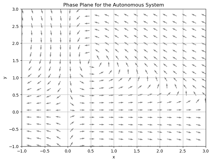
9. Plot a phase plane for the system

\[x' = x(7-2x)-4xy\]

\[y' = -y+2xy.\]

import numpy as np
import matplotlib.pyplot as plt

# Set the range of values for x and y
x = np.linspace(-1, 3, 20)
y = np.linspace(-1, 3, 20)

# Create a grid of points (x, y)
X, Y = np.meshgrid(x, y)

# Define the system of equations
dx = X*(7 - 2*X) - 4*X*Y
dy = -Y + 2*X*Y

# Normalize the arrows to have the same length
N = np.sqrt(dx**2 + dy**2)
dx = dx/N
dy = dy/N

# Create the quiver plot
plt.figure(figsize=(8, 6))
plt.quiver(X, Y, dx, dy, color='gray')

plt.title('Phase Plane for the Autonomous System')
plt.xlabel('x')
plt.ylabel('y')
plt.xlim([-1, 3])
plt.ylim([-1, 3])
plt.grid(True)
plt.show()

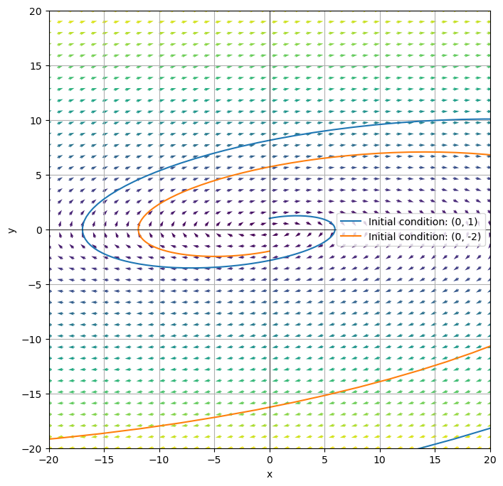
10. Consider the two-dimensional homogeneous linear system

\[\begin{split} x' = \begin{bmatrix} 0 & 10 \\ -1 & 2 \end{bmatrix}x. \end{split}\]

Find eigenvalues and their respective eigenvectors and use this information to plot a phase plane with two sample solution curves.

The eigenvalues of \(A\) are \(\lambda = 1 \pm 3i\). The eigenvector associated to \(\lambda = 1+3i\) is \(\begin{bmatrix} 1-3i \\ 1 \end{bmatrix}\) and the eigenvector associated to \(\lambda = 1-3i\) is \(\begin{bmatrix} 1+3i \\ 1 \end{bmatrix}\).

import numpy as np
import matplotlib.pyplot as plt
from scipy.integrate import solve_ivp

# Define the system of equations
def system(t, state):
    x, y = state
    dx = 10*y
    dy = -1*x + 2*y
    return [dx, dy]

# Set up the grid
Y, X = np.mgrid[-20:20:40j, -20:20:40j]
DX, DY = system(None, [X, Y])

# Normalize vectors to a consistent length for visualization
M = (np.hypot(DX, DY))
M[M == 0] = 1.
DX /= M
DY /= M

fig, ax = plt.subplots(figsize=(8, 8))

# Plot the vector field using quiver
ax.quiver(X, Y, DX, DY, M, pivot='mid')

# Define the eigenvalues and eigenvectors
lambda1 = 1-3j
lambda2 = 1+3j
v1 = np.array([1+3j, 1])
v2 = np.array([1-3j, 1])

x = np.linspace(-10, 10, 800)

# Plot solution curves for two initial conditions
t_span = [-10, 10]
t_eval = np.linspace(t_span[0], t_span[1], 1000)

for initial_condition in [(0, 1), (0, -2)]:
    sol = solve_ivp(system, t_span, initial_condition, t_eval=t_eval)
    ax.plot(sol.y[0], sol.y[1],label=f'Initial condition: {initial_condition}')

ax.set_xlabel('x')
ax.set_ylabel('y')
ax.grid(True)
ax.axvline(0, color='black',linewidth=0.5)
ax.axhline(0, color='black',linewidth=0.5)
plt.xlim([-20, 20])
plt.ylim([-20, 20])
ax.legend()
plt.show()

11. Consider the nonlinear autonomous system

\[x' = x(5-x)-4xy\]

\[y' = y(3-y)-2xy.\]

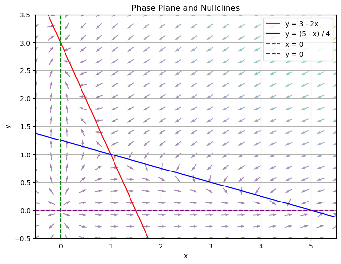
Find the nullclines and equilibrium points and plot a phase plane. Then find the linearization at each equilibrium solution, and if possible, use that linearization to describe the qualitative behavior near each equilibrium solution.

To find the nullclines, we set each equation equal to zero.

When \(x'=0\): \(x(5-x-4y)=0 \rightarrow x=0 \text{ or } y= \dfrac{5-x}{4}\). These are the \(x'\) nullclines.

When \(y'=0\): \(y(3-y-2x)=0 \rightarrow y=0 \text{ or } y= 3-2x\). These are the \(y'\) nullclines.

Notice that from these nullclines, we can also find the equilibrium solutions, by figuring out the intersection points. Notice that \((0,0)\) is an equilibrium solution corresponding to \(x=0\), \(y=0\). \((0,3)\) is an eqilibrium solution corresponding to \(x=0\), \(y=3-2x\). \((5,0)\) is an equilibrium solution corresponding to \(y=\dfrac{5-x}{4}\), \(y=0\). The last equilibrium solution is \((1,1)\), which corresponds to \(y= \dfrac{5-x}{4}\), \(y=3-2x\).

import numpy as np
import matplotlib.pyplot as plt

# Define the system of equations
def system(x, y):
    dx = x * (5 - x) - 4 * x * y
    dy = y * (3 - y) - 2 * x * y
    return dx, dy

# Create an x, y grid
y, x = np.mgrid[-0.5:3.5:20j, -0.5:5.5:20j]

# Calculate dx, dy for the vector field
dx, dy = system(x, y)

# Normalize the arrows so their size represents their speed
M = (np.hypot(dx, dy))                           
M[M == 0] = 1.                                 
dx /= M                                        
dy /= M

plt.figure(figsize=(8, 6))

# Plot the vector field using quiver
plt.quiver(x, y, dx, dy, M, pivot='mid', alpha=0.5)

# Create an x vector
x = np.linspace(-0.5, 5.5, 400)

# Define nullclines
y1 = 3 - 2 * x
y2 = (5 - x) / 4

# Plot nullclines
plt.plot(x, y1, 'r', label="y = 3 - 2x")
plt.plot(x, y2, 'b', label="y = (5 - x) / 4")

# Also plot x=0 and y=0
plt.axvline(0, color='green', linestyle='--', label="x = 0")
plt.axhline(0, color='purple', linestyle='--', label="y = 0")

# Labels and legends
plt.xlabel('x')
plt.ylabel('y')
plt.legend()

# Set the x and y axis cutoffs
plt.ylim([-0.5,3.5])
plt.xlim([-0.5,5.5])

plt.grid(True)
plt.title('Phase Plane and Nullclines')
plt.show()

Now we want to find the Jacobian Matrix, \(J(x,y)\).

\[\begin{split}J(x,y) = \begin{bmatrix} \dfrac{\partial }{\partial x}(5x-x^2-4xy) & \dfrac{\partial }{\partial y}(5x-x^2-4xy) \\ \dfrac{\partial }{\partial x}(3y-y^2-2xy) & \dfrac{\partial }{\partial y}(3y-y^2-2xy) \end{bmatrix} = \begin{bmatrix} 5-2x-4y & -4x \\ -2y & 3-2y-2x \end{bmatrix}\end{split}\]

So the linearization of \((0,0)\) is

\[\begin{split} \begin{bmatrix} x' \\ y' \end{bmatrix} = J(0,0) \begin{bmatrix} x-0 \\ y-0 \end{bmatrix} = \begin{bmatrix} 5 & 0 \\ 0 & 3 \end{bmatrix}\begin{bmatrix} x \\ y \end{bmatrix}\end{split}\]

So the linearization of \((0,3)\) is

\[\begin{split} \begin{bmatrix} x' \\ y' \end{bmatrix} = J(0,3) \begin{bmatrix} x-0 \\ y-3 \end{bmatrix} = \begin{bmatrix} -2 & 0 \\ -6 & -3 \end{bmatrix}\begin{bmatrix} x \\ y-3 \end{bmatrix}\end{split}\]

So the linearization of \((5,0)\) is

\[\begin{split} \begin{bmatrix} x' \\ y' \end{bmatrix} = J(5,0) \begin{bmatrix} x-5 \\ y-0 \end{bmatrix} = \begin{bmatrix} -5 & -20 \\ 0 & -7 \end{bmatrix}\begin{bmatrix} x-5 \\ y \end{bmatrix}\end{split}\]

So the linearization of \((1,1)\) is

\[\begin{split} \begin{bmatrix} x' \\ y' \end{bmatrix} = J(1,1) \begin{bmatrix} x-1 \\ y - 1 \end{bmatrix} = \begin{bmatrix} -1 & -4 \\ -2 & -1 \end{bmatrix}\begin{bmatrix} x-1 \\ y - 1 \end{bmatrix}\end{split}\]

From this analysis, we would expect \((0,0)\) to behave like a source. We would expect \((0,3)\) to behave like a sink. We would expect \((5,0)\) to behave like a sink. We would expect \((1,1)\) to behave like a sink and a source (depending on where we approach it).

Section 6 Solutions

1. By hand show that the Laplace transforms of \(\cos(bt)\) and \(\sin(bt)\) are the functions listed in the chart. *Recall: Euler’s formula says \(e^{i(bt)} = \cos(bt)+i\sin(bt)\).

   \[\mathcal{L}(e^{ibt}) = \int_{0}^{\infty} e^{-st}e^{ibt} \mathrm{d}t\]
   \[\mathcal{L}(e^{ibt}) = \int_{0}^{\infty} e^{-st}(\cos(bt)) \mathrm{d}t + i \displaystyle{\int_0^{\infty} e^{-st}(\sin(bt)) \mathrm{d}t}\]

\[= \mathcal{L}(\cos(bt)) + i \mathcal{L}(\sin(bt))\]

Since

\[\mathcal{L}(e^{ibt}) = \dfrac{1}{s-ib} \dfrac{s+ib}{s+ib} = \dfrac{s+ib}{s^2+b^2} = \dfrac{s}{s^2+b^2} + i \dfrac{b}{s^2+b^2},\]

we know that \(\mathcal{L}(\cos(bt)) = \dfrac{s}{s^2-b^2}\) and \(\mathcal{L}(\sin(bt)) = \dfrac{b}{s^2-b^2} \) for \(s >|ib|\).

2. Show that the Laplace transform of \(f'(t)\) is \(sF(s)-f(0)\).

We know

\[\mathcal{L}(f'(t)) = \int_{0}^{\infty} e^{-st}f'(t) \mathrm{d}t.\]

Applying integration by parts yields

\[ \mathcal{L}(f'(t)) = \lim_{r \to \infty} \left( e^{-st}f(t) \right) \bigg|_{t=0}^{t=r} + s \int_{0}^{\infty} e^{-st} f(t) dt. \]

Notice that

\[ s\int_{0}^{\infty} e^{-st}f(t) \mathrm{d}t = F(s), \lim_{r \rightarrow \infty} \left( e^{-sr}f(r)\right) = 0 \]

because \(f(t)\) is of expontential order. Thus

\[\mathcal{L}(f'(t)) = [0-f(0)]+sF(s) = sF(s)-f(0).\]

3. Show that the Laplace transform of \(f''(t)\) is \(s^2F(s)-sf(0)-f'(0)\).

We know

\[\mathcal{L}(f''(t)) = \int_{0}^{\infty} e^{-st}f''(t) \mathrm{d}t.\]

Applying integration by parts yields

\[\mathcal{L}(f''(t)) = \lim_{r \rightarrow \infty} \left( e^{-st}f'(t)\right)\bigg|_{t=0}^{t=r} + s\int_{0}^{\infty} e^{-st}f'(t) \mathrm{d}t.\]

Notice that

\[ s\int_{0}^{\infty} e^{-st}f'(t) \mathrm{d}t = s(sF(s)-f(0)), \lim_{r \rightarrow \infty} \left( e^{-sr}f'(r)\right) = 0 \]

because \(f'(t)\) is of expontential order. Thus

\[\mathcal{L}(f''(t)) = [0-f'(0)]+s(sF(s)-f(0)) = s^2F(s)-sf(0)-f'(0).\]

4. Show that the function \(g(x) = e^{t^2}\) does not have a Laplace transform.

\[\mathcal{L}(e^{t^2}) = \int_{0}^{\infty} e^{-st}e^{t^2} \mathrm{d}t = \infty\]

Thus, the Laplace transform is not defined.

5. Find the Laplace transform of \(f(t) = 8+3e^{2t}-\cos(6t)\).

\[\mathcal{L}(f(t)) = 8 \mathcal{L(1)} + 3\mathcal{L}(e^{2t})-\mathcal{L}(\cos(6t))\]

\[= \dfrac{8}{s} + \dfrac{3}{s-2} + \dfrac{s}{s^2+36}.\]

6. Solve the initial value problem

\[x'' + 4x'+3x = 10\cos(t), \quad x(0)=2, \quad x'(0)=3.\]

\[\mathcal{L}(x'' + 4x'+3x) = 10\mathcal{L}(\cos(t))\]

\[\mathcal{L}(x'') + 4\mathcal{L}(x') + 3 \mathcal{L}(x) = 10\mathcal{L}(\cos(t))\]

\[[s^2X(s) - sx(0)-x'(0)]+4[sX(s)-x(0)]+3X(s) = \dfrac{10s}{s^2+1}\]

\[(s^2+4s+3)X(s)-2s-11 = \dfrac{10s}{s^2+1}\]

\[X(s)(s+1)(s+3) = \dfrac{10s}{s^2+1} + \dfrac{(2s+11)(s^2+1)}{(s^2+1)}\]

\[X(s) = \dfrac{2s^3+11s^2+12s+11}{(s^2+1)(s+1)(s+3)}\]

Now use partial fractions

\[\dfrac{2s^3+11s^2+12s+11}{(s^2+1)(s+1)(s+3)} = \dfrac{A}{s+1} + \dfrac{B}{s+3} + \dfrac{Cs+D}{s^2+1}\]

Solving for \(A\), \(B\), \(C\), and \(D\), yields \(A = 2\), \(B=-1\), \(C=1\), and \(D=2\).

Thus \(X(s) = \dfrac{2}{s+1} - \dfrac{1}{s+3} + \dfrac{s+2}{s^2+1}\). Therefore, \(x(t) =2e^{-t}-e^{-35}+\cos(t)+2\sin(t)\).

7. Solve the initial value problem

\[x'' + 2x'+3x = 9t, \quad x(0)=1, \quad x'(0)=2.\]

\[\mathcal{L}(x'' + 2x'+3x) = 9\mathcal{L}(t)\]

\[\mathcal{L}(x'') + 2\mathcal{L}(x') + 3 \mathcal{L}(x) = 9\mathcal{L}(t)\]

\[[s^2X(s) - sx(0)-x'(0)]+2[sX(s)-x(0)]+3X(s) = \dfrac{9}{s^2}\]

\[(s^2+2s+3)X(s)-s-4 = \dfrac{9}{s^2}\]

\[X(s) = \dfrac{s^3+4s^2+9}{(s^2)(s^2+2s+3)}\]

Now use partial fractions

\[\dfrac{s^3+4s^2+9}{(s^2)(s^2+2s+3)} = \dfrac{A}{s} + \dfrac{B}{s^2} + \dfrac{Cs+D}{s^2+2s+3}\]

Solving for \(A\), \(B\), \(C\), and \(D\), yields \(A = -2\), \(B=3\), \(C=3\), and \(D=5\).

Thus \(X(s) = \dfrac{-2}{s} - \dfrac{3}{s^2} + \dfrac{3s+5}{s^2+2s+3}\).

Completing the square of \(s^2+2s+3 = (s+1)^2+\sqrt{2}^2\). So \(\dfrac{3s+5}{s^2+2s+3} = \dfrac{3s+5}{(s+1)^2+\sqrt{2}^2} = 3\dfrac{s+1}{(s+1)^2+\sqrt{2}^2} + \sqrt{2}\dfrac{\sqrt{2}}{(s+1)^2+\sqrt{2}^2}\).

Thus, \(X(s) =\dfrac{-2}{s} - \dfrac{3}{s^2}+3\dfrac{s+1}{(s+1)^2+\sqrt{2}^2} + \sqrt{2}\dfrac{\sqrt{2}}{(s+1)^2+\sqrt{2}^2}\). Therefore, \(x(t) = -2, 3t+3e^{-t}\cos(\sqrt{2}t)+\sqrt{2}e^{-t}\sin(\sqrt{2}t)\).

8. Let \(f(t) = \begin{cases} t & \text{ if } 0 \leq t \leq 2 \\ 0 & \text{ if } t>2 \end{cases}\). Solve the initial value problem

\[x'' + x = f(t), \quad x(0)=0, \quad x'(0)=0.\]

Hint: First rewrite \(f(t)\) using the Heaviside function so that you can take the Laplace transform of both sides.

First note that \(f(t) = t + u(t-2)[-t]\). Then we know

\[\mathcal{L}(x'') + \mathcal{L}(x) = \mathcal{L}(t) - \mathcal{L}(u(t-2)\cdot t)\]

\[s^2X(s)+X(s) = \dfrac{1}{s^2}-e^{-2s}G(s)\]

where \(G(s) = \mathcal{L}(t+2)= \dfrac{1}{s^2}+\dfrac{2}{s}\).

Thus,

\[X(s) = \dfrac{1}{s^2(s^2+1)} - e^{-2s}\dfrac{1}{s^2(s^2+1)} - 2e^{-2s}\dfrac{1}{s(s^2+1)}\]

Using partial fractions we find that \(\dfrac{1}{s^2(s^2+1)} = \dfrac{1}{s^2} - \dfrac{1}{s^2+1}\) and \(\dfrac{1}{s(s^2+1)} = \dfrac{1}{s} - \dfrac{s}{s^2+1}\). This means that

\[X(s) = \dfrac{1}{s^2} - \dfrac{1}{s^2+1}-e^{-2s}\dfrac{1}{s^2} + e^{-2s}\dfrac{1}{s^2+1}-2e^{-2s}\dfrac{1}{s} +2e^{-2s}\dfrac{s}{s^2+1}\]

Therefore,

\[x(t) = t - \sin(t) -u(t-2)[t-2]+u(t-2)\sin(t-2)-2u(t-2)+2u(t-2)\cos(t-2) = t - \sin(t) + u(t-2)[\sin(t-2)+2\cos(t-2)-t].\]