11.9. JNB Lab Solutions#
11.9.1. Chapter Review#
Section 2 Questions#
List the type, order, and parameters of each of the following differential equations. For each ordinary differential equation, determine if it is linear or nonlinear.
\(\dfrac{dy}{dx} +3x^2 = sin(x) + 3\)
ODE, first order, linear (remember, the order depends on the highest derivative, not the power of the independent variable)
\((\dfrac{dy}{dx})^2 +3x^2 = sin(x) + 3\)
ODE, first order, non-linear
\(\dfrac{dy}{dx}k +3x^2 k = y\,sin(x) + 3\)
ODE, first order, linear, parameter \(k\)
\(\dfrac{d^2y}{dx^2} +3x^2 = sin(x) + 3\)
ODE, second order, linear
\(\frac{\partial w}{\partial u} + \frac{\partial^2 w}{\partial v^2} = u\)
PDE, second order
\(\frac{\partial w}{\partial u} + \frac{\partial w}{\partial v} = u^2\)
PDE, first order
\(\dfrac{dt}{dv}t = tan(t) +9\)
ODE, first order, non-linear
\(\dfrac{dt}{dv}v = tan(t) +9\)
ODE, first order, linear
\( \)
Show that \(y = e^{2t}\) is a solution for all \(t\) to \(y''+y = 5y\).
\(y'=2e^{2t}, y''=4e^{2t}\); plugging these in, we get \( 4e^{2t}+e^{2t}=5e^{2t} \), which is true.
Show that \(y = te^{5t}\) is a solution for all \(t\) to \(y''-10y'=-25y\).
\( y'= 5te^{5t} +e^{5t}, y''=25te^{5t}+10e^{5t} \); plugging these in, we get \( 25te^{5t}+10e^{5t}-10(5te^{5t}+e^{5t})=-25(te^{5t}) \). Simplifying the left side will yield \( -25te^{5t} \), which is the same as the right side.
Show that \(y = sin(3t)+cos(3t) + t^3 -6\) is a solution for all \(t\) to \(y'''+9y' = 27t^2+6\).
\( y'= 3cos(3t)-3sin(3t)+3t^2, y''=-9sin(3t)-9cos(3t)+6t, y'''=-27cos(3t)+27sin(3t)+6 \). Plugging these values into the equation yields: \( -27cos(3t)+27sin(3t)+6 + 9(3cos(3t)-3sin(3t)+3t^2) = 27t^2+6 \); simplifying the left side gives us \( 27t^2+6 \), which is the same as the right side.
Show that \(y = 12t^2+t^4\) is a solution for all \(t\) to \((y'+y'')-(y'''+y^{(4)}) = y-t^4+4t^3\).
\( y'= 24t+4t^3, y''= 24+12t^2, y'''= 24t, y^{(4)}=24 \). Plugging these in yields: \( 24t+4t^3+24+12t^2-(24t+24)=(12t^2+t^4)-t^4+4t^3 \). Both sides reduce to \( 4t^3+12t^2 \), so \( y= 12t^2+t^4\) is a solution for all \(t\) to the initial equation.
Section 3 Questions#
Solve the separable equations:
\( \dfrac{dx}{dt} = \dfrac{1}{t}e^{-2x} \)
\(x= \dfrac{ln(2ln(t)+C)}{2}\)
\( \dfrac{dx}{dt} = \dfrac{-1}{x^2t^2} \)
\(x = \sqrt[3]{\dfrac{3}{t}+C}\)
\( \dfrac{dy}{dx} = cos^2(y)e^{x^2}2x \)
\( y = arctan(e^{x^2} +C) \)
\( \dfrac{1}{x}-\dfrac{dx}{dt}=x^{-1}\dfrac{1}{sec(t)} \)
\(x = \pm\sqrt{2t-2sin(t)+C} \)
Solve the linear equations using the method of integrating factors (\(\mu(t) = e^{P(t)}\)):
\( t\dfrac{dx}{dt} = sin(t) -x \)
\(\mu = e^{ln(t)}= t\)
\( x=\dfrac{-cos(t)+C}{t} \)
\( \dfrac{dx}{dt} + x 4t^3 = \dfrac{1}{t e^{t^4}} \)
\( \mu = e^{t^4} \)
\( x= \dfrac{ln(t)+C}{e^{t^4}} \)
\( \dfrac{dy}{dx} + \dfrac{y}{x} = \dfrac{1}{x+x^3} \)
\(\mu = e^{ln(x)}=x \)
\( y= \dfrac{arctan(x)+C}{x} \)
\( \dfrac{dy}{dx}x + \dfrac{-2y}{x^2} = xe^{-x^{-2}}sec(x)tan(x) \)
\(\mu = e^{x^{-2}} \)
\( y = \dfrac{sec(x)+C}{e^{x^{-2}}} \)
Find the equilibrium solutions and draw the phase lines for the following functions. Classify each equilibrium solution.
\( y'=(y-6)(y+7) \)
Solutions: \( y = 6, -7 \)
Classification: \( y = 6\): source. \( y = -7\): sink.
\( y'= y^3-8y^2+12y \)
Solutions: \( y = 0, 2, 6 \)
Classification: \(y = 0\): source. \(y = 2\): sink. \(y = 6\): source.
\( y'= y(y^2-1) \)
Solutions: \(y = 0, 1, -1\)
Classification: \(y=-1\): source. \(y=0\): sink. \(y=1\): source.
\( y'= y^2(y^2-1) \)
Solutions: \(y = 0, 1, -1 \)
Classification: \(y=-1\): sink. \(y=0\): node. \(y=1\): source.
Below are hand-drawn phase lines for all four equations.
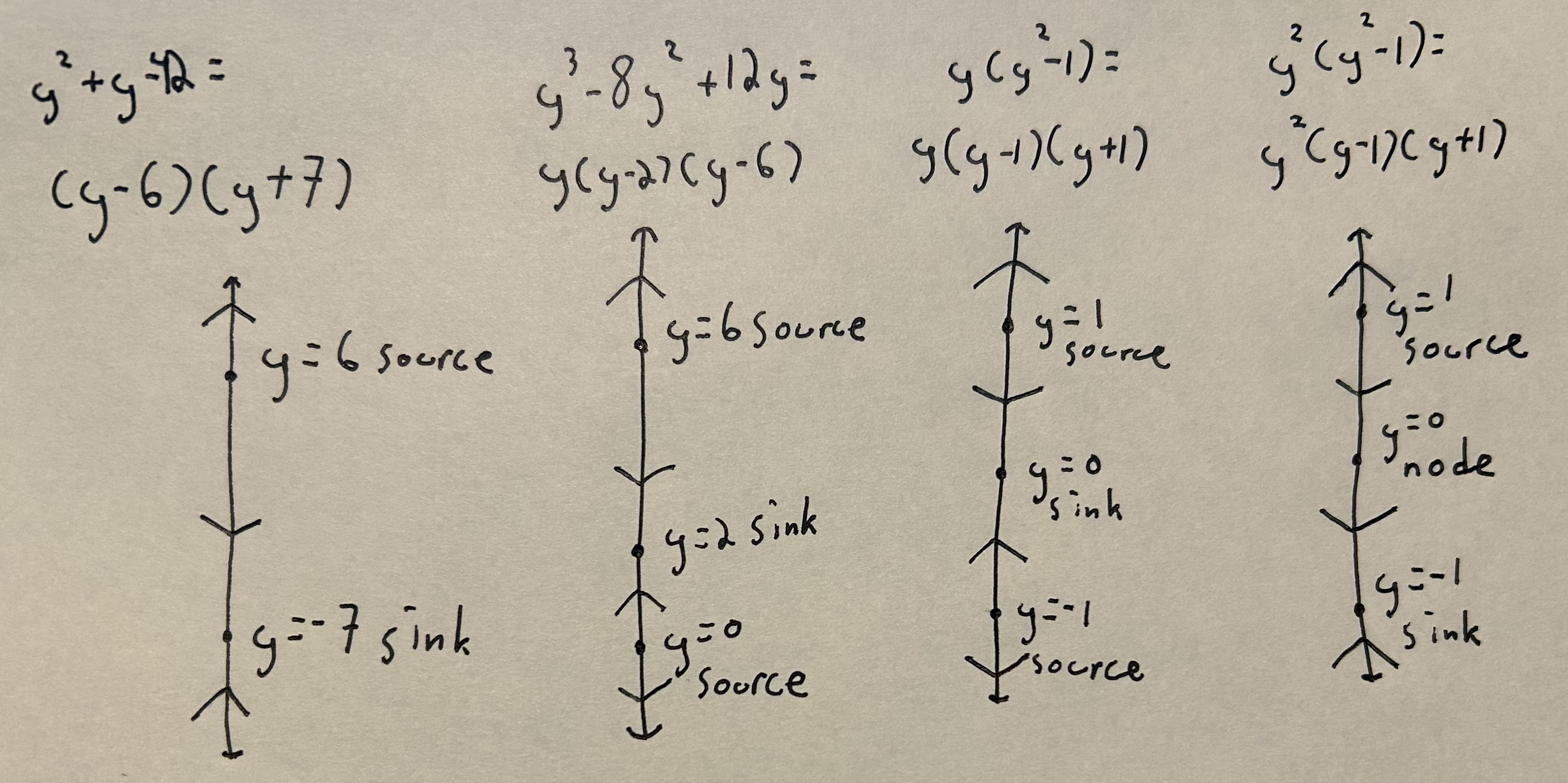
Note
Take note of how the repeated root of 0 in the last problem compared with the one before changes the classification of the equilibrium solutions. The phase lines can be drawn by hand or created using the sample code in Section 3.4 of the chapter (Autonomous Equations).
Section 4 Questions#
Solve the initial value problem:
\( x'' - x' -42x = 0 \); \( x'(0) = 0\), \( x''(0) = 1\)
\( x = \dfrac{e^{7t}}{91}+\dfrac{e^{-6t}}{78} \)
\( x''-14x'+48x=0 \); \(x'(0)=0\), \(x''(0)=5\)
\( x=\dfrac{5}{16}e^{8t}-\dfrac{5}{12}e^{6t} \)
\( x''+6x'+9x=0, x'(0)=0, x''(0)=9 \)
\( x=-e^{-3t}-3e^{-3t}t \)
\( x''+16x'+64x=0, x'(0)=0, x''(0)=8 \)
\( x=-\dfrac{e^{-8t}}{8}-e^{-8t}t \)
\( x''+4x'+8x=0, x'(0)=0, x''(0)=4 \)
\( x= -\dfrac{e^{-2t}}{2}(cos(2t)+sin(2t)) \)
\( x''+10x'+30x=0, x'(0)= 0, x''(0)= 30 \)
\( x= e^{-5t}(-cos(\sqrt{5}t)-\sqrt{5}sin(\sqrt{5}t)) \)
Solve the non-homogeneous equations:
\( x''-9x'+20x=-10 \)
\( c_1e^{5t}+c_2e^{4t}-\dfrac{1}{2} \)
\( x''-9x'+20x=20t^2 \)
\( c_1e^{5t}+c_2e^{4t} +t^2+\dfrac{9t}{10}+\dfrac{61}{200} \)
\( x''-9x'+20x=e^{3t} \)
\( c_1e^{5t}+c_2e^{4t}+\dfrac{1}{2}e^{3t} \)
\( x''-9x'+20x=e^{5t} \)
\( c_1e^{5t}+c_2e^{4t} +te^{5t} \)
Solve the non-homogeneous equations:
\( x''+4x'+4x =sin(t)\)
\( c_1e^{-2t}+c_2e^{-2t}t+\dfrac{3}{25}sin(t)-\dfrac{4}{25}cos(t) \)
\( x''+4x'+4x =8t^2 \)
\( c_1e^{-2t}+c_2e^{-2t}t+ 2t^2-4t+3\)
Section 5 Questions#
Rewrite as a system of first order equations:
\( x'''+3x''+12x'+x=sin(t)+e^{3t} \)
Define new variables: \(x_1=x\), \(x_2=x'\), \(x_3=x''\)
From this, we see that \(x_1'=x_2\), \(x_2'=x_3\), and so we can rewrite the original equation as:
Solution: \(x_3'=-x_1-12x_2-3x_3+sin(t)+e^{3t}\)
Test the following sets of vectors for linear independence:
\(\biggl\{\begin{bmatrix} 2e^{t} \\ e^{12t} \end{bmatrix}, \begin{bmatrix} 12e^{2t} \\ 6e^{12t} \end{bmatrix}\biggr\}\)
independent
\(\biggl\{\begin{bmatrix} 5e^{3t} \\ 6e^{6t} \end{bmatrix}, \begin{bmatrix} 10e^{3t} \\ 12e^{6t} \end{bmatrix}\biggr\}\)
dependent
\(\biggl\{\begin{bmatrix} 3t \\ 1 \end{bmatrix}, \begin{bmatrix} 3t \\ tan^2(t) \end{bmatrix}, \begin{bmatrix} 6t \\ sec^2(t) \end{bmatrix} \biggr\}\)
dependent: \(1+tan^2(t)=sec^2(t)\), \(so, v_1+v_2-v_3=0\)
Find the eigenvalues and eigenvectors:
\(\begin{bmatrix} 3&0 \\ 0&4 \end{bmatrix}\)
Eigenvalues: \( r_1=3 \), \(r_2=4\)
Eigenvectors: \( v_1=\begin{bmatrix} 1\\0\end{bmatrix} \), \(v_2 = \begin{bmatrix}0\\1\end{bmatrix} \)
\(\begin{bmatrix} 6&2 \\ -2&2 \end{bmatrix}\)
Eigenvalue: \( r=4 \)
Eigenvector: \( v= \begin{bmatrix} -1\\1 \end{bmatrix} \)
\(\begin{bmatrix} 3&2 \\ -9&-3 \end{bmatrix}\)
Eigenvalues: \( r_1 = 3i \), \( r_2 = -3i \)
Eigenvectors: \( v_1= \begin{bmatrix} \dfrac{-1-i}{3}\\1 \end{bmatrix} \), \(v_2=\begin{bmatrix} \dfrac{-1+i}{3}\\1 \end{bmatrix} \)
Solve the linear systems where \( x'=Ax \) of differential equations, for each choice of A:
\(A=\begin{bmatrix} 3&-2 \\ 4&9 \end{bmatrix}\)
Eigenvalues: \(r_1=5, r_2=7\)
Eigenvectors: \(v_1=\begin{bmatrix} -1 \\ 1 \end{bmatrix}\), \(v_2=\begin{bmatrix} -\dfrac{1}{2} \\ 1 \end{bmatrix}\)
Solution: \(x=c_1e^{5t}\begin{bmatrix} -1 \\ 1 \end{bmatrix}+ c_2e^{7t}\begin{bmatrix} -1 \\ 2 \end{bmatrix}\)
\(A=\begin{bmatrix} 5&-2 \\ 2&1 \end{bmatrix}\)
Eigenvalue: \(r=3\)
Eigenvector: \(\begin{bmatrix} 1 \\ 1 \end{bmatrix}\)
Solution: \(x= c_1e^{3t}\begin{bmatrix} 1 \\ 1 \end{bmatrix}+ c_2e^{3t}(t\begin{bmatrix} 1 \\ 1 \end{bmatrix}+\begin{bmatrix} \dfrac{1}{2} \\ 0 \end{bmatrix})\)
\(A=\begin{bmatrix} 6&13 \\ -4&-6 \end{bmatrix}\)
Eigenvalues: \( \pm4i\)
Eigenvectors: for \(+4i\): \(v_1= \begin{bmatrix} \dfrac{-3-2i}{2} \\ 1 \end{bmatrix} \); for \(-4i\): \(v_2= \begin{bmatrix} \dfrac{-3+2i}{2} \\ 1 \end{bmatrix}\)
Solution: \(x= c_1(cos(4t)\begin{bmatrix} -3 \\ 2 \end{bmatrix}-sin(4t)\begin{bmatrix} -2 \\ 0 \end{bmatrix}) +c_2(cos(4t)\begin{bmatrix} -2 \\ 0 \end{bmatrix}+sin(4t)\begin{bmatrix} -3 \\ 2 \end{bmatrix}) \)
Find the nullclines, equilibrium solutions, and linearization of the system:
\( x'=x(1-x)-4xy \); \( y'=y(2-y)-3xy \)
\(x'\) nullclines: \(x=0\), \(y=\dfrac{1-x}{4}\)
\(y'\) nullclines: \(y=0\), \(y=2-3x\)
Equilibrium solutions: \( (0,0),(1,0),(0,2),(\dfrac{7}{11},\dfrac{1}{11}) \)
Linearization: \((0,0)\): \( \begin{bmatrix} 1&0 \\ 0&2 \end{bmatrix}\begin{bmatrix} x \\ y \end{bmatrix} \); \((1,0)\): \(\begin{bmatrix} -1&-4 \\ 0&-1 \end{bmatrix}\begin{bmatrix} x-1 \\ y \end{bmatrix} \); \((0,2)\): \(\begin{bmatrix} -7&0 \\ -6&-2 \end{bmatrix}\begin{bmatrix} x \\ y-2 \end{bmatrix} \); \( (\dfrac{7}{11}, \dfrac{1}{11}) \): \(\begin{bmatrix} -\dfrac{7}{11}&-\dfrac{28}{11} \\ -\dfrac{3}{11}&-\dfrac{1}{11} \end{bmatrix}\begin{bmatrix} x-\dfrac{7}{11} \\ y-\dfrac{1}{11} \end{bmatrix} \)
Section 6 Questions#
Solve the following Laplace Transforms by hand, using the formula \(\mathcal{L}(f(t)) = \int_{0}^{\infty} e^{-st}f(t) \mathrm{d}t \equiv F(s).\)
\( f(t)= sin(t)\)
\(\dfrac{1}{s^2+1}\)
\( f(t)= cos(t)\)
\( \dfrac{s}{s^2+1} \)
\( f(t)=8t+e^{3t}+cos(3t) \)
\( \dfrac{8}{s^2}+\dfrac{1}{s-3}+\dfrac{s}{s^2+9} \)
Find the inverse Laplace Transforms of the following functions:
\( \mathcal{L}(x)=-\dfrac{14}{s^3}+\dfrac{1}{s^2+49} \)
\(-7t^2+\dfrac{1}{7}sin(7t)\) (Hint: you can multiply \(\dfrac{1}{s^2+49}\) by 7 in the numerator, then by \(\dfrac{1}{7}\) out front to get it into the right form to use the formula for \(sin(t)\))
\( \mathcal{L}(x)= \dfrac{s+9}{(s+2)(s+3)}\)
Partial fractions: \( \dfrac{s+9}{(s+2)(s+3)}= \dfrac{A}{s+2} +\dfrac{B}{s+3} \); \(A=7\), \(B=-6\). Therefore, \( \mathcal{L}(x)= 7e^{-2t}-6e^{-3t}\)
\( \mathcal{L}(x)= x''+12x=3, x(0)=x'(0)=0 \)
Take the Laplace Transform of both sides:
Solve for \(X(s)\):
Partial Fraction Decomposition:
Inverse Laplace Transform:
Express the following functions in terms of the unit step function, then take the Laplace Transform:
\( f(t) = \begin{cases} 0 & \text{ if } t < 2 \\ 1 & \text{ if } t>2 \end{cases} \)
\( u(t-2) \); \( \mathcal{L}(x)= \dfrac{e^{-2s}}{s} \)
\( f(t) = \begin{cases} 2 & \text{ if } 0< t < 1 \\ 3 & \text{ if } 1<t<2 \\ 4 & \text{ if } t>2 \end{cases} \)
\( 2+u(t-1)+u(t-2) \); \( \mathcal{L}(x)= \dfrac{2}{s}+ \dfrac{e^{-s}}{s}+\dfrac{e^{-2s}}{s} \)
11.9.2. Python Questions#
import sympy as sp
First and second order equations#
Solve \( \dfrac{dy}{dx}= 3x^2y \) using Sympy code
x = symbols("x")
y = Function("y")
eq1 = - y(x).diff(x) + 3* x**2 *y(x)
dsolve(eq1)
Solve \(y'' + 3y = 0\)
t = symbols("t")
y = Function("y")
eq2 = y(t).diff(t).diff(t)+3*y(t)
dsolve(eq2)
Solve \( \dfrac{dy}{dx}= cos(x)+3y \)
x = symbols("x")
y = Function("y")
eq3 = - y(x).diff(x) + sp.cos(x) + 3*y(x)
dsolve(eq3)
Solve \( x''+2x'+2x=12 \)
t = symbols("t")
x = Function("x")
eq4 = 12 -2*x(t) -2*x(t).diff(t) -x(t).diff(t).diff(t)
dsolve(eq4)
Solve \( \dfrac{dy}{dx} = \dfrac{1}{(1+x^2)}y^2 \)
x = symbols("x")
y = Function("y")
eq5 = -y(x).diff(x) + y(x)**(2) / (1 + x**2)
dsolve(eq5)
Direction Fields#
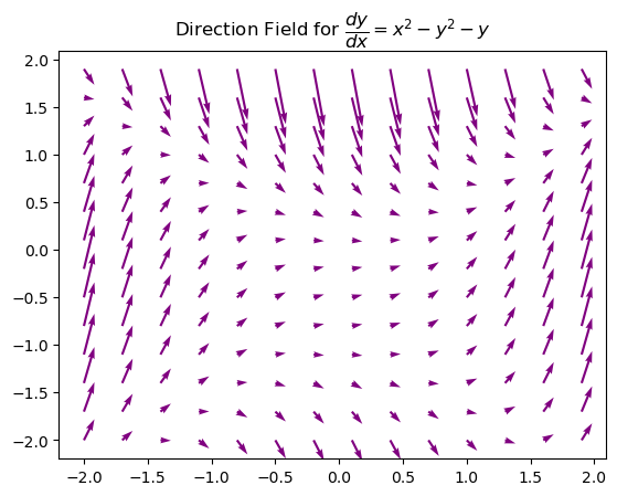
Use Python code to plot the direction fields:
\( \dfrac{dy}{dx}= x^2-y^2-y \)
import numpy as np
import matplotlib.pyplot as plt

nx, ny = .3, .3
x = np.arange(-2,2,nx)
y = np.arange(-2,2,ny)

#Create a rectangular grid with points
X,Y = np.meshgrid(x,y)

#Define the functions
dy = X**2 - Y**2 - Y
dx = np.ones(dy.shape)

#Plot
plt.quiver(X,Y,dx,dy,color='purple')
plt.title('Direction Field for $ \dfrac{dy}{dx} = x^2 - y^2 - y $ ')
plt.show()
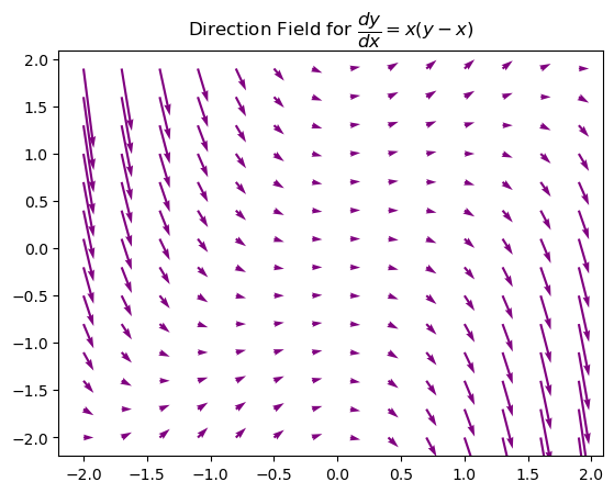
\( \dfrac{dy}{dx}= x(y-x) \)
import numpy as np
import matplotlib.pyplot as plt

nx, ny = .3, .3
x = np.arange(-2,2,nx)
y = np.arange(-2,2,ny)

#Create a rectangular grid with points
X,Y = np.meshgrid(x,y)

#Define the functions
dy = X*(Y-X)
dx = np.ones(dy.shape)

#Plot
plt.quiver(X,Y,dx,dy,color='purple')
plt.title('Direction Field for $ \dfrac{dy}{dx} = x(y - x) $')
plt.show()
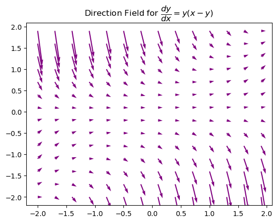
\( \dfrac{dy}{dx}= y(x-y) \)
import numpy as np
import matplotlib.pyplot as plt

nx, ny = .3, .3
x = np.arange(-2,2,nx)
y = np.arange(-2,2,ny)

#Create a rectangular grid with points
X,Y = np.meshgrid(x,y)

#Define the functions
dy = Y*(X-Y)
dx = np.ones(dy.shape)

#Plot
plt.quiver(X,Y,dx,dy,color='purple')
plt.title('Direction Field for $ \dfrac{dy}{dx} = y(x - y) $ ')
plt.show()
Phase Planes and Phase Portraits#
Edit the code from Section 5.4 to plot the phase planes, then find the equilibrium solutions:
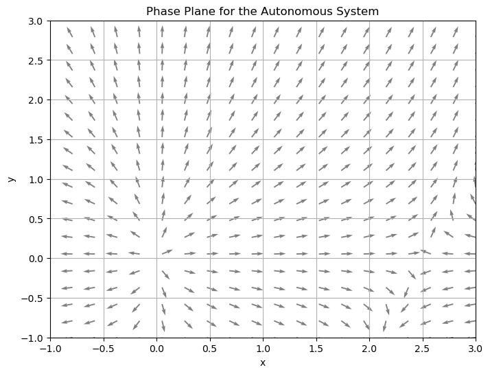
\( \dfrac{dx}{dt}= x (x + 3) - 2xy \), \( \dfrac{dy}{dt} = y (3y - 8) - xy \)
Equilibrium solutions: \( (0,0), (0,\dfrac{8}{3}), (-3,0), (7,5) \)
import numpy as np
import matplotlib.pyplot as plt

# Set the range of values for x and y
x = np.linspace(-1, 3, 20)
y = np.linspace(-1, 3, 20)

# Create a grid of points (x, y)
X, Y = np.meshgrid(x, y)

# Define the system of equations
dx = X*(X + 3) - 2*X*Y
dy = Y*(3*Y - 8) - X*Y

# Normalize the arrows to have the same length
N = np.sqrt(dx**2 + dy**2)
dx = dx/N
dy = dy/N

# Create the quiver plot
plt.figure(figsize=(8, 6))
plt.quiver(X, Y, dx, dy, color='gray')

plt.title('Phase Plane for the Autonomous System')
plt.xlabel('x')
plt.ylabel('y')
plt.xlim([-1, 3])
plt.ylim([-1, 3])
plt.grid(True)
plt.show()

\( \dfrac{dx}{dt} = x (5 - 2x) + xy\), \( \dfrac{dy}{dt} = y (y + 1) + y\)
Equilibrium solutions: \( (0,0), (0,-2), (\dfrac{5}{2}, 0), (1.5,-2) \)
import numpy as np
import matplotlib.pyplot as plt

# Set the range of values for x and y
x = np.linspace(-1, 3, 20)
y = np.linspace(-1, 3, 20)

# Create a grid of points (x, y)
X, Y = np.meshgrid(x, y)

# Define the system of equations
dx = X*(5 - 2*X) + X*Y
dy = Y*(Y + 1) + Y

# Normalize the arrows to have the same length
N = np.sqrt(dx**2 + dy**2)
dx = dx/N
dy = dy/N

# Create the quiver plot
plt.figure(figsize=(8, 6))
plt.quiver(X, Y, dx, dy, color='gray')

plt.title('Phase Plane for the Autonomous System')
plt.xlabel('x')
plt.ylabel('y')
plt.xlim([-1, 3])
plt.ylim([-1, 3])
plt.grid(True)
plt.show()
Edit the code from Section 5.4 to plot the phase portraits of the same systems
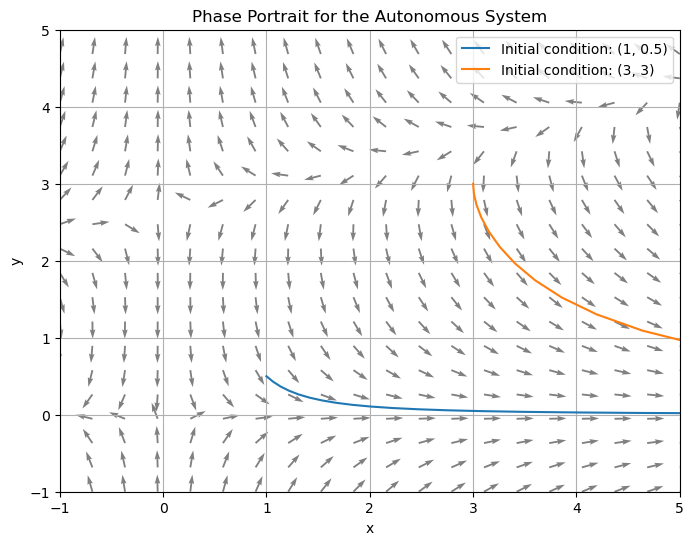
3. \( \dfrac{dx}{dt}= x (x + 3) - 2xy \), \( \dfrac{dy}{dt} = y (3y - 8) - xy \)
import numpy as np
import matplotlib.pyplot as plt
from scipy.integrate import odeint

# Define the range of values for x and y
x = np.linspace(-1, 5, 20)
y = np.linspace(-1, 5, 20)

# Create a grid of points (x, y)
X, Y = np.meshgrid(x, y)

# Define the system of equations
U = X*(X + 3) - 2*X*Y
V = Y*(3*Y - 8) - X*Y

# Normalize the arrows to have the same length
N = np.sqrt(U**2 + V**2)
U = U/N
V = V/N

# Define the system for odeint
def dFdt(F, t):
    return [F[0]*(F[0] + 3) - 2*F[0]*F[1], F[1]*(3*F[1] - 8) -F[0]*F[1] ]

# Set the time points where the solution is computed
t = np.linspace(-10, 10, 1000)  # Negative times are included here

# Set a collection of initial conditions
initial_conditions = [(1, 0.5), (3, 3)]

# Create the quiver plot
plt.figure(figsize=(8, 6))
plt.quiver(X, Y, U, V, color='gray')

# Loop over each initial condition and plot the solution curve
for ic in initial_conditions:
    F = odeint(dFdt, ic, t)
    plt.plot(F[:, 0], F[:, 1], label=f'Initial condition: {ic}')

plt.title('Phase Portrait for the Autonomous System')
plt.xlabel('x')
plt.ylabel('y')
plt.xlim([-1, 5])
plt.ylim([-1, 5])
plt.grid(True)
plt.legend()
plt.show()
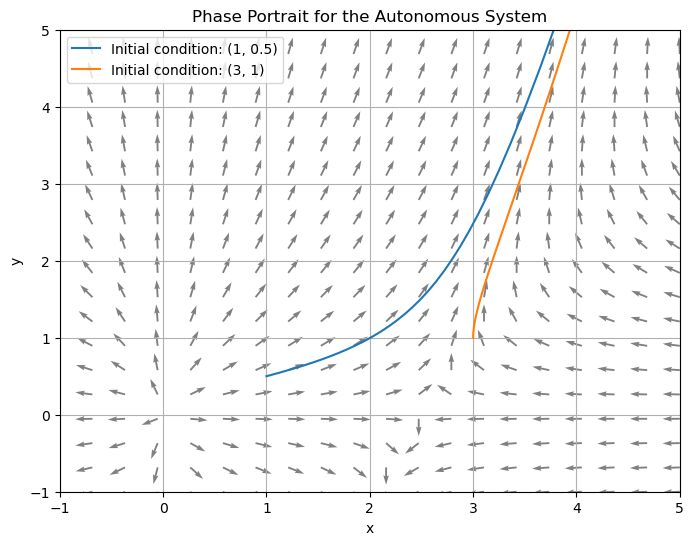
\( \dfrac{dx}{dt} = x (5 - 2x) + xy\), \( \dfrac{dy}{dt} = y (y + 1) + y\)
import numpy as np
import matplotlib.pyplot as plt
from scipy.integrate import odeint

# Define the range of values for x and y
x = np.linspace(-1, 5, 20)
y = np.linspace(-1, 5, 20)

# Create a grid of points (x, y)
X, Y = np.meshgrid(x, y)

# Define the system of equations
U = X*(5 - 2*X) + X*Y
V = Y*(Y + 1) + Y

# Normalize the arrows to have the same length
N = np.sqrt(U**2 + V**2)
U = U/N
V = V/N

# Define the system for odeint
def dFdt(F, t):
    return [F[0]*(5 - 2*F[0]) + F[0]*F[1], F[1]*(F[1] + 1) + F[1] ]

# Set the time points where the solution is computed
t = np.linspace(-10, 10, 1000)  # Negative times are included here

# Set a collection of initial conditions
initial_conditions = [(1, 0.5), (3, 1)]

# Create the quiver plot
plt.figure(figsize=(8, 6))
plt.quiver(X, Y, U, V, color='gray')

# Loop over each initial condition and plot the solution curve
for ic in initial_conditions:
    F = odeint(dFdt, ic, t)
    plt.plot(F[:, 0], F[:, 1], label=f'Initial condition: {ic}')

plt.title('Phase Portrait for the Autonomous System')
plt.xlabel('x')
plt.ylabel('y')
plt.xlim([-1, 5])
plt.ylim([-1, 5])
plt.grid(True)
plt.legend()
plt.show()
Nullclines#
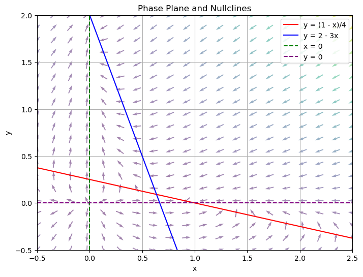
Plot the nullclines for the following system (from Chapter review section 5):
\( x'=x(1-x)-4xy \); \( y'=y(2-y)-3xy \)
import numpy as np
import matplotlib.pyplot as plt

# Define the system of equations
def system(x, y):
    dx = x * (1 - x) - 4 * x * y
    dy = y * (2 - y) - 3 * x * y
    return dx, dy

# Create an x, y grid
y, x = np.mgrid[-0.5:2:20j, -0.5:2.5:20j]

# Calculate dx, dy for the vector field
dx, dy = system(x, y)

# Normalize the arrows so their size represents their speed
M = (np.hypot(dx, dy))
M[M == 0] = 1.
dx /= M
dy /= M

plt.figure(figsize=(8, 6))

# Plot the vector field using quiver
plt.quiver(x, y, dx, dy, M, pivot='mid', alpha=0.5)

# Create an x vector
x = np.linspace(-0.5, 2.5, 200)

# Define nullclines
y1 = (1 - x)/4
y2 = 2 - 3 * x

# Plot nullclines
plt.plot(x, y1, 'r', label="y = (1 - x)/4")
plt.plot(x, y2, 'b', label="y = 2 - 3x")

# Also plot x=0 and y=0
plt.axvline(0, color='green', linestyle='--', label="x = 0")
plt.axhline(0, color='purple', linestyle='--', label="y = 0")

# Labels and legends
plt.xlabel('x')
plt.ylabel('y')
plt.legend()

# Set the x and y axis cutoffs
plt.ylim([-0.5,2])
plt.xlim([-0.5,2.5])

plt.grid(True)
plt.title('Phase Plane and Nullclines')
plt.show()
Laplace Transforms#
import numpy as np
import matplotlib.pyplot as plt
import sympy as sym
from sympy.abc import s,t
Find the Laplace Transforms of the following functions:
\( f(t)= 3t^2+cos(3t)+12 \)
f = 3*t**2 + sym.cos(3*t) + 12  # define your function with respect to t
F = sym.laplace_transform(f, t, s)  # sym.laplace_transform_(function, func_var, out_var)

print(F)  # returns F(s) and convergence interval
(s/(s**2 + 9) + 12/s + 6/s**3, 0, True)
\( f(t)= \dfrac{1}{2}sin(t)+ 5t\)
f = 1/2 * sym.sin(t) + 5*t  # define your function with respect to t
F = sym.laplace_transform(f, t, s)  # sym.laplace_transform_(function, func_var, out_var)

print(F)  # returns F(s) and convergence interval
(0.5/(s**2 + 1) + 5/s**2, 0, True)
Find the Inverse Laplace Transforms of the following functions:
\( f(t)= \dfrac{7}{s}+ \dfrac{720}{s^7} + \dfrac{1}{(5s^2+\dfrac{1}{5})} \)
# Define the inverse Laplace transform function
def invL(F):
    return sym.inverse_laplace_transform(F, s, t)

F= 7/s + 720/s**7 + 1/(5*s**2+1/5)
print(invL(F))
t**6*Heaviside(t) + 1.0*sin(0.2*t)*Heaviside(t) + 7*Heaviside(t)
\( f(t)= \dfrac{2}{2s-1}+\dfrac{72}{s^4} \)
# Define the inverse Laplace transform function
def invL(F):
    return sym.inverse_laplace_transform(F, s, t)

F= 2/(2*s-1) + 72/s**4
print(invL(F))
12*t**3*Heaviside(t) + exp(t/2)*Heaviside(t)
Solve the IVP:
\( y'' + 2y'+3y = 9t, \, y(0)=1, \, y'(0)=2 \)
import numpy as np
from sympy import *
import sympy as sym
from sympy.abc import s,t

# Define the inverse Laplace transform function
def invL(F):
    return sym.inverse_laplace_transform(F, s, t)
#Solve the IVP
s=sym.symbols('s')
t=sym.symbols('t')
f=sym.Function('s')
F=sym.laplace_transform(f(t),t,s)
g=t
G=sym.laplace_transform(g,t,s)
print('Transform of t is', G[0])

# Transform the equation  and solve for Y=L(y)
eq=Eq((s**2) * F - s - 2 + 2 *s* F -2 + 3* F -9*G[0],0 )
Y = solve(eq, F)
print('Transform of y is',Y)

# Take the inverse transform
print('y=',invL(Y[0]))
Transform of t is s**(-2)
Transform of y is [(s**3 + 4*s**2 + 9)/(s**2*(s**2 + 2*s + 3))]
y= ((3*t - 2)*exp(t) + sqrt(2)*sin(sqrt(2)*t) + 3*cos(sqrt(2)*t))*exp(-t)*Heaviside(t)