import numpy as np
9.3. Matrices and Determinants#
9.3.1. Matrix Algebra#
This section focuses on matrix algebra and its properties. We will also explore how operations involving matrices are connected to linear systems.
Matrices#
Consider matrix \(A\), which is an \(m \times n\) matrix with \(m\) rows and \(n\) columns:
The entry in the \(i\)th row and \(j\)th column is referred to as the \((i,j)\)-entry of matrix \(A\). Entries with the same row and column index (\(a_{i,i}\) for any \(i\)) are called diagonal entries of \(A\). The \(i\)th column of \(A\), denoted as \(a_i\), represents a vector in \(\mathbb{R}^m\). We can represent matrix \(A\) in a compact form by its columns:
or by its entries:
A matrix whose entries are all zero is called a zero matrix, denoted by \(0\). The size of a zero matrix is usually clear from the context.
An \(n \times n\) matrix is called:
the identity matrix, denoted by \(I_n\), if it has 1 on the diagonal and 0 everywhere else.
a diagonal matrix if it has all nondiagonal entries equal to zero. Identity matrices are diagonal.
an upper triangular matrix if it has all entries below the diagonal equal to zero.
a lower triangular matrix if it has all entries above the diagonal equal to zero.
a triangular matrix if it is either upper triangular or lower triangular.
Example 1
Let
As we have seen before, we use NumPy arrays to represent A. Note that each list in the array represents a row of A.
import numpy as np

A = np.array([[0, 2, -1],[2, 3, 1]])
print('A =\n', A)
A =
 [[ 0  2 -1]
 [ 2  3  1]]
\(A\) is a \(2 \times 3\) matrix. The following cell shows how to find the size of \(A\):
#Size of A

print('A has ', A.shape[0],  'rows, and', A.shape[1],  'columns')
A has 2 rows, and 3 columns
We can also print rows and columns of \(A\):
print('The first row of A is ', A[0,:])

print(30*'*')

print('\nThe second row of A is ', A[1,:])

print(30*'*')

print('\nThe first column of A is ', A[:,0])

print(30*'*')

print('\nThe second column of A is ', A[:,1])

print(30*'*')

print('\nThe third column of A is ', A[:,2])
The first row of A is  [ 0  2 -1]
******************************

 The second row of A is  [2 3 1]
******************************

 The first column of A is  [0 2]
******************************

 The second column of A is  [2 3]
******************************

 The third column of A is  [-1  1]
The following cell shows how to generate an identity matrix of an arbitrary size:
# 3x3 identity matrix
I_3 = np.eye(3)

print('I_3 = \n \n', I_3)

# 4x4 identity matrix I_4
I_4 = np.eye(4)

print('\n I_4 = \n \n', I_4)

# 5x5 identity matrix I_5
I_5 = np.eye(5)

print('\n I_5 = \n \n', I_5)
I_3 =

 [[1. 0. 0.]
 [0. 1. 0.]
 [0. 0. 1.]]

 I_4 =

 [[1. 0. 0. 0.]
 [0. 1. 0. 0.]
 [0. 0. 1. 0.]
 [0. 0. 0. 1.]]

 I_5 =

 [[1. 0. 0. 0. 0.]
 [0. 1. 0. 0. 0.]
 [0. 0. 1. 0. 0.]
 [0. 0. 0. 1. 0.]
 [0. 0. 0. 0. 1.]]
Let’s have more examples:
B = np.array([[1, 2, 3],[4, 5, 6]])
print('B =\n', B)


#Size of B

print('\n B has ', B.shape[0],  'rows, and', B.shape[1],  'columns')

#The second column of B

print('\n The second column of B is ', B[:,1])

print(30*'*')

C = np.array([[0, 2] ,[2, 3],[5, -2]])
print('\n C = \n', C)


#Size of C

print('\n C has ', C.shape[0],  'rows, and', C.shape[1],  'columns')


#Print the columns of C

for i in range(C.shape[1]):
    print('\n The', i+1, '-th column of C is ', B[:,i])
B =
 [[1 2 3]
 [4 5 6]]

 B has  2 rows, and 3 columns

 The second column of B is  [2 5]
******************************

 C =
 [[ 0  2]
 [ 2  3]
 [ 5 -2]]

 C has  3 rows, and 2 columns

 The 1 -th column of C is  [1 4]

 The 2 -th column of C is  [2 5]
Basic Algebraic Operations#
The arithmetic operations defined for vectors can be extended to matrices:
Two matrices \(A\) and \(B\) are equal if they have the same size and entries.
The sum of matrices is defined for matrices of the same size:
let \(A = (a_{ij})\) and \(B = (b_{ij})\) be two \(m \times n\) matrices. Then \(A+B\) is an \(m \times n\) matrix whose entries are the sums of the corresponding entries of \(A\) and \(B\):
The scalar product \(cA\) for a scalar \(c \in \mathbb{R}\) and a matrix \(A\) is a matrix of the same size as \(A\) whose entries are \(c\) times the entries of \(A\):
Theorem 1 (properties of sum and scalar product)
Let \(A\), \(B\), and \(C\) have the same size, and let \(c\) and \(d\) be real numbers.
\(A+B = B+A\)
\((A+B)+C = A+(B+C)\)
\(A+ 0 = A\)
\(c(A+B) = cA + cB\)
\((c+d)A = cA + dA\)
\(c(dA)=(cd)A\)
Example 2:
Consider the matrices in Example 1. Compute the following:
\(3A-B\)
\(A+C\)
Solution:
#1

3*A-B
array([[-1,  4, -6],
       [ 2,  4, -3]])
\(A+C\) is not defined because \(A\) and \(C\) are not of the same size:
#2.
A + C
---------------------------------------------------------------------------
ValueError                                Traceback (most recent call last)
Cell In[8], line 2
      1 #2.
----> 2 A + C

ValueError: operands could not be broadcast together with shapes (2,3) (3,2)
Matrix Product#
Let \(A\) be an \(m \times n\) and \(B\) be an \(n \times p\) matrix. The product AB is an \(m\times p\) matrix whose columns are \(Ab_1, Ab_2, \dots, Ab_p\):
We can also describe the matrix product by the entries: the (\(ij\))-entry of \(AB\) is the product of the \(i\)th-row of \(A\) and the \(j\)th column of \(B\) in the following way:
The product \(BA\) is not defined if \(p\neq m\) (the neighboring dimensions do not match).
Example 3
Let
\(A = \begin{bmatrix} 1 & 2 & 3 \\ 4 & 5 & 6 \end{bmatrix}\) and \(B = \begin{bmatrix} 1 & 2 \\ 3 & 4 \\ 5 & 6\\ \end{bmatrix}\).
Compute \(AB\) and \(BA\).
Solution:
\(A\) is a \(2 \times 3\) and B is a \(3 \times 2\) matrix; so the product is defined. In Python, we use the symbol @ to compute the matrix product
#A
A = np.array([[1,2,3],[4,5,6]])

#B
B = np.array([[1,2],[3,4],[5,6]])

#Compute the matrix product
AB = A @ B

print(AB)
[[22 28]
 [49 64]]
Now let’s compute \(BA\):
#Compute the product BA
BA = B @ A

print(BA)
[[ 9 12 15]
 [19 26 33]
 [29 40 51]]
Example 4
Let
The matrix product \(AC\) is not defined because the number of columns in matrix \(A\) does not match the number of rows in matrix \(C\). If we proceed with computing \(AC\) we will get:
C = np.array([[1, 2, 3, 4], [4, 5, 6, 7]])

# Compute AC
AC = A @ C

print(AC)
---------------------------------------------------------------------------
ValueError                                Traceback (most recent call last)
Cell In[11], line 4
      1 C = np.array([[1, 2, 3, 4], [4, 5, 6, 7]])
      3 # Compute AC
----> 4 AC = A @ C
      6 print(AC)

ValueError: matmul: Input operand 1 has a mismatch in its core dimension 0, with gufunc signature (n?,k),(k,m?)->(n?,m?) (size 2 is different from 3)
Power of Square Matrices
We can raise a square matrix \(A\) to the power of a natural number using matrix multiplication. The matrix power is a fundamental idea in several linear algebra applications such as the long-term behavior of discrete dynamical systems.
Example 5
Let \(M = BA\) where \(A\) and \(B\) are matrices in Example 3. Compute \(M^{4}\).
#C
M = BA
#Compute C^4
M4 = M @ M @ M @ M

print('C^4 =\n ', M4 )
C^4 =
  [[ 5447976  7470048  9492120]
 [11879096 16288144 20697192]
 [18310216 25106240 31902264]]
Interestingly, computing the power of diagonal matrices is relatively straightforward.
Example 6:
Let’s consider the matrix \(A = \begin{bmatrix} 2 & 0\\ 0 & 5 \end{bmatrix}\). We can observe the pattern for computing powers of \(A\):
\(A^2 = \begin{bmatrix} 2^2 & 0\\ 0 & 5^2 \end{bmatrix} = \begin{bmatrix} 4 & 0\\ 0 & 25 \end{bmatrix}\)
\(A^3 = \begin{bmatrix} 2^3 & 0\\ 0 & 5^3 \end{bmatrix} = \begin{bmatrix} 8 & 0\\ 0 & 125 \end{bmatrix}\)
\(A^4 = \begin{bmatrix} 2^4 & 0\\ 0 & 5^4 \end{bmatrix} = \begin{bmatrix} 16 & 0\\ 0 & 625 \end{bmatrix}\)
We can observe that \(A^k\) is a diagonal matrix of the same size with the diagonal elements being obtained by raising the corresponding diagonal elements of \(A\) to the power of \(k\).
A = np.array([[2,0],[0,5]])

A2 = A @ A
A2
array([[ 4,  0],
       [ 0, 25]])
A3 = A2 @ A
A3
array([[  8,   0],
       [  0, 125]])
Theorem 2 (Properties of matrix product)
Let \(A\) be an \(m\times n\) matrix, and let \(B\) and \(C\) be matrices of the same size for which the following sum and product operations are defined:
\(A(BC) = (AB)C\)
\(A(B+C) = AB + AC\)
\((B+C)A = BA + CA\)
\(r(AB) = (rA)B = A(rB)\) for any scalar \(r\in \mathbb{R}\).
\(I_mA = AI_n = A\)
Recall that \(I_n\) is the \(n \times n\) identity matrix.
Numerical Note#
NumPy provides two other methods (built-in functions) to compute the matrix product: numpy.dot and numpy.matmul.
They are both used to compute the product of two arrays (e.g., vectors, matrices, and even higher dimensional).
(1). If \(A\) and \(B\) are vectors (1-D arrays), they both perform the dot product of vectors (which we will define in section 6)
(2). If \(A\) and \(B\) are non-vector matrices (2-D arrays), they both perform matrix multiplication, but using numpy.matmul(A,B) or A @ B is preferred.
(3) For scalar \(r\in \mathbb{R}\) numpy.dot(r,B) is scalar product r*B. But numpy.malmal(r,B) and r @ B are not defined
Example 7
Let A, B, and C be the matrices defined in Example 3. Let’s explore the differences between the above operations:
import numpy as np

#A
A = np.array([[1,2,3],[4,5,6]])

#B
B = np.array([[1,2],[3,4],[5,6]])


# for matrices (2D-arrays) of compatible size all methods return matrix product

print('\n A@B = \n', A@B)

print(10*'*')

print('\n np.dot(A,B) = \n', np.dot(A,B))

print(10*'*')

print('\n np.matmul(A,B) = \n', np.matmul(A,B))
 A@B =
 [[22 28]
 [49 64]]
**********

 np.dot(A,B) =
 [[22 28]
 [49 64]]
**********

 np.matmul(A,B) =
 [[22 28]
 [49 64]]
# for vectors (1D arrays) dot and matmul return the dot product
C = [1,2,3]
D = [4,5,6]

print('\n np.dot(C,D) = \n', np.dot(C,D))

print(10*'*')

print('\n np.matmul(C,D) = \n', np.matmul(C,D))
 np.dot(C,D) =
 32
**********

 np.matmul(C,D) =
 32
# C@D is not defined for vectors

print('\n A@B = \n', C @ D)
---------------------------------------------------------------------------
TypeError                                 Traceback (most recent call last)
Cell In[17], line 3
      1 # C@D is not defined for vectors
----> 3 print('\n A@B = \n', C @ D)

TypeError: unsupported operand type(s) for @: 'list' and 'list'
# If one argument is a real number, dot returns the scalar product
print('\n np.matmul(2,B) = \n', np.dot(A,2))
 np.matmul(2,B) =
 [[ 2  4  6]
 [ 8 10 12]]
# If one argument is a real number  @ and matmul are not defined
2 @ B
---------------------------------------------------------------------------
ValueError                                Traceback (most recent call last)
Cell In[19], line 2
      1 # If one argument is a real number  @ and matmul are not defined
----> 2 2 @ B

ValueError: matmul: Input operand 0 does not have enough dimensions (has 0, gufunc core with signature (n?,k),(k,m?)->(n?,m?) requires 1)
np.matmul (2,B)
---------------------------------------------------------------------------
ValueError                                Traceback (most recent call last)
Cell In[20], line 1
----> 1 np.matmul (2,B)

ValueError: matmul: Input operand 0 does not have enough dimensions (has 0, gufunc core with signature (n?,k),(k,m?)->(n?,m?) requires 1)
Exercises
Which pair of the following matrices can be multiplied? Compute their matrix product.
Find two matrices \(A\) and \(B\) such that the products \(AB\) and \(BA\) are defined but \(AB \neq BA\).
Given
find a nonzero matrix \(C\) for which
9.3.2. Transpose, Inverse and Trace of matrices#
In this section, we will continue studying the basic operators on the set of matrices, focusing on the transpose, inverse, and trace of a square matrix.
Transpose of a matrix#
Given an \(m\times n\) matrix \(A\), the transpose of \(A\) is the \(n\times m\) matrix denoted by \(A^T\), whose columns are the corresponding rows of \(A\).
Example 1
If
then
In Python, we can either use narray.T or narray.transpose() to find the transpose of a matrix.
import numpy as np

M = np.array([[1,2],[3, 4],[5,6]])

#Compute the the transpose of M
M_T = M.T

print("M = ", '\n', M, '\n\n', "M_T = ",'\n', M_T)
M =
 [[1 2]
 [3 4]
 [5 6]]

 M_T =
 [[1 3 5]
 [2 4 6]]
#Compute the the transpose of M
M_transpose = M.transpose()

print("M = ", '\n', M, '\n\n', "M_T = ",'\n', M_transpose)
M =
 [[1 2]
 [3 4]
 [5 6]]

 M_T =
 [[1 3 5]
 [2 4 6]]
Note that transpose and T both have different effect on a list and a list of lists:
# transpose of a list of lists

np.array([[1,2,3]]).transpose()
array([[1],
       [2],
       [3]])
# does not effect 1D array
np.array([1,2,3]).transpose()
array([1, 2, 3])
Inverse of a square matrix#
An \(n\times n\) matrix \(A\) is called invertible if there exists an \(n\times n\) matrix \(B\) such that \(AB = BA = I_n\). In this case, \(B\) is referred to as the inverse of \(A\), denoted as \(A^{-1}\). It is important to note that not all matrices are invertible.
Theorem 3
Let \(A= \begin{bmatrix} a & b \\ c & d\\ \end{bmatrix}\). If \(ad-bc \neq 0\), then \(A\) is invertible, and its inverse is given by:
\(ad-bc\) is called the determinant of matrix A. The determinant plays a crucial role in determining the invertibility of a square matrix. If the determinant is zero, i.e., \(ad-bc = 0\), then matrix A is not invertible. Determinants of matrices will be discussed in the next section, where we will explore their properties and computation methods.
Example 2
Find the inverse of \(M= \begin{bmatrix} 1 & 2 \\ 3 & 4\\ \end{bmatrix}\).
Find the inverse of \(N= \begin{bmatrix} 1 & 2 \\ 2 & 4\\ \end{bmatrix}\).
Solution:
Let’s write a Python code that computes the inverse of a \(2\times 2\) matrix:
M = np.array([[1, 2], [3, 4]])
N = np.array([[1, 2], [2, 4]])

# Compute the inverse
def inverse_matrix(matrix):
    a, b = matrix[0]
    c, d = matrix[1]

    det = a * d - b * c

    if det == 0:
        print(matrix, "is not invertible")
    else:
        D = 1 / det
        inverse = np.zeros((2, 2))
        inverse[0, 0] = D * d
        inverse[0, 1] = -D * b
        inverse[1, 0] = -D * c
        inverse[1, 1] = D * a

        return(inverse)
inverse_matrix(M)
array([[-2. ,  1. ],
       [ 1.5, -0.5]])
inverse_matrix(N)
[[1 2]
 [2 4]] is not invertible
Theorem 4 (properties of the inverse matrix)
Let \(A\) and \(B\) be two invertible \(n\times n\) matrices.
\((A^{-1})^{-1} = A\)
\((AB)^{-1} = B^{-1}A^{-1}\)
\((A^{T})^{-1} = (A^{-1})^{T}\)
Theorem 5 (computing the inverse of a square matrix)
An \(n\times n\) matrix \(A\) is invertible if and only if it is row equivalent to the identity matrix \(I_n\).
We can use this theorem to find the inverse of a matrix using the row reduction method: set up the augmented matrix \([A|I_n]\) and perform row operations until the left side of the augmented matrix becomes the identity matrix \(I_n\). If this is achieved, then the right side of the augmented matrix will be the inverse of \(A\). Otherwise, if the left side does not become \(I_n\), then the matrix \(A\) is not invertible.
Example 3
Find the inverse of \(M= \begin{bmatrix} 0 & 1 & 2\\ 1 & 0 & 3\\ 4 & -3 & 8 \end{bmatrix}\).
Solution Lets set up the augmented matrix and find its RREF:
# matrix M

M = np.array([[0,1,2], [1,0,3], [4, -3, 8]])
M
array([[ 0,  1,  2],
       [ 1,  0,  3],
       [ 4, -3,  8]])
# identity matrix I_3

I3 = np.eye(3)
I3
array([[1., 0., 0.],
       [0., 1., 0.],
       [0., 0., 1.]])
# Augmented matrix [A,I_3]

A = np.concatenate((M, I3), axis = 1)
A
array([[ 0.,  1.,  2.,  1.,  0.,  0.],
       [ 1.,  0.,  3.,  0.,  1.,  0.],
       [ 4., -3.,  8.,  0.,  0.,  1.]])
Now lets call row operations
# Elementry row operations:

# Swap two rows

def swap(matrix, row1, row2):

    copy_matrix=np.copy(matrix).astype('float64')

    copy_matrix[row1,:] = matrix[row2,:]
    copy_matrix[row2,:] = matrix[row1,:]

    return copy_matrix


# Multiple all entries in a row by a nonzero number


def scale(matrix, row, scalar):
    copy_matrix=np.copy(matrix).astype('float64')
    copy_matrix[row,:] = scalar*matrix[row,:]
    return copy_matrix

# Replacing a row by the sum of itself and a multiple of another

def replace(matrix, row1, row2, scalar):
    copy_matrix=np.copy(matrix).astype('float64')
    copy_matrix[row1] = matrix[row1]+ scalar * matrix[row2]
    return copy_matrix
A_1 = swap(A, 0, 1)
A_1
array([[ 1.,  0.,  3.,  0.,  1.,  0.],
       [ 0.,  1.,  2.,  1.,  0.,  0.],
       [ 4., -3.,  8.,  0.,  0.,  1.]])
A_2 = replace(A_1, 2, 0, -4)
A_2
array([[ 1.,  0.,  3.,  0.,  1.,  0.],
       [ 0.,  1.,  2.,  1.,  0.,  0.],
       [ 0., -3., -4.,  0., -4.,  1.]])
A_3 = replace(A_2, 2, 1, 3)
A_3
array([[ 1.,  0.,  3.,  0.,  1.,  0.],
       [ 0.,  1.,  2.,  1.,  0.,  0.],
       [ 0.,  0.,  2.,  3., -4.,  1.]])
A_4 = scale(A_3, 2, 1/2)
A_4
array([[ 1. ,  0. ,  3. ,  0. ,  1. ,  0. ],
       [ 0. ,  1. ,  2. ,  1. ,  0. ,  0. ],
       [ 0. ,  0. ,  1. ,  1.5, -2. ,  0.5]])
A_5 = replace(A_4, 1, 2, -2)
A_5
array([[ 1. ,  0. ,  3. ,  0. ,  1. ,  0. ],
       [ 0. ,  1. ,  0. , -2. ,  4. , -1. ],
       [ 0. ,  0. ,  1. ,  1.5, -2. ,  0.5]])
A_6 = replace(A_5, 0, 2, -3)
A_6
array([[ 1. ,  0. ,  0. , -4.5,  7. , -1.5],
       [ 0. ,  1. ,  0. , -2. ,  4. , -1. ],
       [ 0. ,  0. ,  1. ,  1.5, -2. ,  0.5]])
We can see that the resulting matrix is in the form \([I_3, B]\). Thus, \(B= \begin{bmatrix} -4.5 & 7 & -1.5\\ -2 & 4 & -1 \\ 1.5 & -2 & 0.5 \\ \end{bmatrix}\) is the inverse of \(M\).
Remark We can also use an np.linalg.inv() function, from NumPy linear algebra submodule, to find an inverse of a matrix:
np.linalg.inv(M)
array([[-4.5,  7. , -1.5],
       [-2. ,  4. , -1. ],
       [ 1.5, -2. ,  0.5]])
Theorem 6 (The Invertible Matrix Theorem)
Let \(A\) be an \(n\times n\) matrix. The following statements are equivalent:
\(A\) is an invertible matrix.
\(A\) is row equivalent to \(I_n\).
The equation \(A\vec{x}=0\) has only the trivial solution (\(\vec{x} = \mathbf{0}\)).
The columns of \(A\) form a linearly independent set.
The equation \(A\vec{x}=\vec{b}\) has a unique solution (\(\vec{x} = A^{-1}\vec{b}\)).
The columns of \(A\) span \(\mathbb{R}^n\).
Example 4
Find the solution set of the following linear systems:
\(M\vec{x}=0\), where \(M\) is the matrix from Example 7.
\(M\vec{x}=\vec{b}\), where \(M\) is the matrix from Example 7 and \(\vec{b}=\begin{bmatrix} 1 \\ 2 \\ 3 \end{bmatrix}\).
Solution:
Since \(M\) is invertible, by the Invertible Matrix Theorem part (3), the only solution to \(M\vec{x}=0\) is the zero vector \(\vec{x}=\mathbf{0}\).
By IMT part (5), the only solution to \(M\vec{x}=\vec{b}\) is \(\vec{x}=M^{-1}\vec{b}\). In Example 7, we computed the inverse of \(M\):
\(A^{-1} = \begin{bmatrix} -4.5 & 7 & -1.5 \\ -2 & 4 & -1 \\ 1.5 & -2 & 0.5 \end{bmatrix}\)
In the following cell, we use \(B\) to represent \(A^{-1}\) to simplify notation:
B = np.array([[-4.5, 7, -1.5], [-2, 4, -1], [1.5, -2, 0.5]])

b = np.array ([[1], [2], [3]])

#compute Bb

x = B @ b
x
array([[ 5.],
       [ 3.],
       [-1.]])
M = np.array([[0,1,2], [1,0,3], [4,-3,8]])

#compute Mx

Mx= M @ x
Mx
array([[1.],
       [2.],
       [3.]])
which is \(\vec{b}\).
Trace of Square Matrices#
The trace of an \(n\times n\) matrix \(A\), denoted by \(Tr(A)\) or \(tr(A)\), is defined as the sum of the elements on its main diagonal:
Theorem 7 (properties of the trace)
Let \(A\) and \(B\) be two \(n\times n\) matrices, and \(c \in \mathbb{R}\). Then we have the following:
Trace of sum: \(Tr(A + B) = Tr(A) + Tr(B)\)
Trace of scalar product: \(Tr(cA) = c \cdot Tr(A)\)
Trace of identity matrix: \(Tr(I_n) = n\)
Trace of product: \(Tr(AB) = Tr(BA)\)
The trace can also be seen as a function from the set of \(n\times n\) matrices to real numbers. It can be shown that there is only one function that satisfies the above conditions.
Example 5
Let \( M = \begin{bmatrix} 0 & 1 & 2\\ 1 & 0 & 3\\ 4 & -3 & 8 \end{bmatrix}. \)
Then: \( Tr(M) = 0 + 0 + 8 = 8. \)
For large matrices, we can use numpy.trace() to compute the trace. The following code generates a random \(5\times 5\) matrix and computes its trace:
# generate a 5x5 matrix
A = np.random.rand(5, 5)
print(A)


#compute the trace
Tr_A = np.trace(A)
print('\n Tr(A) = ', Tr_A)
[[0.34123286 0.3788517  0.62749816 0.49779428 0.85625537]
 [0.49841636 0.64059001 0.97192421 0.82065731 0.73171872]
 [0.93029465 0.82685801 0.34255562 0.22621385 0.40893711]
 [0.20730845 0.35221413 0.95709886 0.62781555 0.49836643]
 [0.75311689 0.22947177 0.40015054 0.20169886 0.86231891]]

 Tr(A) =  2.814512956289748
Exercises
Suppose
a. Compute \(A^T\).
b. Is \(AA^T\) invertible?
c. Is \(A^TA\) invertible?
The trace is invariant under cyclic permutations, i.e., for three matrices we have \(Tr(ABC) = Tr(BCA) = Tr(CAB)\), where \(A\) is an \(n\times p\) matrix, \(B\) is a \(p\times m\) matrix, and \(C\) is an \(m \times n\) matrix. Using Example 9, generate three matrices \(A\), \(B\), and \(C\) such that the product \(ABC\) makes sense, and verify that:
9.3.3. Determinant#
This section introduces the determinants of matrices and explores some of their properties, applications, and computation methods. The determinant of a square matrix is a useful concept in linear algebra and has many theoretical and practical roles, including:
Determining the invertibility of a matrix.
Determining the linear dependency of a set of vectors.
Computing the area of parallelograms or the volume of parallelepipeds.
Solving linear systems (Cramer’s rule).
Finding the inverse of an invertible matrix.
Note that applications (4) and (5) are based on Cramer’s rule, which is a theoretical tool but not an efficient computational method. We won’t discuss Cramer’s rule.
Cofactor expansion#
In the previous section, we defined the determinant of a \(2\times 2\) matrix as \(det(A) = ad-bc\), where \(A = \begin{bmatrix} a & b \\ c & d \end{bmatrix}\). To extend this definition to larger matrices, we follow a recursive approach. For example, to find the determinant of a \(3\times 3\) matrix, we can use \(2\times 2\) determinants.
Let \(A = \begin{bmatrix} a_{11} & a_{12} & a_{13} \\ a_{21} & a_{22} & a_{23} \\ a_{31} & a_{32} & a_{33} \end{bmatrix}\) be a general \(3\times 3\) matrix. For any entry \(a_{ij}\), let \(A_{ij}\) denote a \(2\times 2\) submatrix of \(A\) defined by removing the row and column of \(A\) that contain \(a_{ij}\). For example, \(A_{12} = \begin{bmatrix} a_{21} & a_{23} \\ a_{31} & a_{33} \end{bmatrix}\) and \(A_{23} = \begin{bmatrix} a_{11} & a_{13} \\ a_{31} & a_{33} \end{bmatrix}\).
Example 1
Write a Python code that prints all submatrices of
Solution:
M = np.array([[1,2,3],[4,5,6],[7,8,9]])
M
array([[1, 2, 3],
       [4, 5, 6],
       [7, 8, 9]])
for j in range (3):
    for i in range (3):
        submatrix = np.delete( (np.delete(M, i , 0)), j ,1)
        print (' \n M(',i,j, ') = \n \n', submatrix)
        print(30*"*")
 M( 0 0 ) =

 [[5 6]
 [8 9]]
******************************

 M( 1 0 ) =

 [[2 3]
 [8 9]]
******************************

 M( 2 0 ) =

 [[2 3]
 [5 6]]
******************************

 M( 0 1 ) =

 [[4 6]
 [7 9]]
******************************

 M( 1 1 ) =

 [[1 3]
 [7 9]]
******************************

 M( 2 1 ) =

 [[1 3]
 [4 6]]
******************************

 M( 0 2 ) =

 [[4 5]
 [7 8]]
******************************

 M( 1 2 ) =

 [[1 2]
 [7 8]]
******************************

 M( 2 2 ) =

 [[1 2]
 [4 5]]
******************************
The determinant of \(A\), expanded over the first row, is defined as:
Here \(|A_{ij}|\) represents the determinant of the \(A_{ij}\). Note that choosing a different row or column would give the same value. For example, using the second row:
Similarly, using the second column:
Example 2
Compute the determinant of
Solution:
Let’s write Python code that computes the determinant of a \(3\times 3\) matrix:
M = np.array([[0,1,2],[1,0,3],[4,-3,8]])
# Computes a 2x2 determinant
def det2(matrix):

    if matrix.shape == (2, 2):
        return matrix[0,0] * matrix[1,1] - matrix[0,1] * matrix[1,0]
    else:
        print("Please enter a 2x2 matrix")

# Computes the 3x3 determinat over a given row

def det3(matrix, row):
    if matrix.shape == (3, 3) and row in range(3):
        det = 0
        for j in range(3):
            submatrix = np.delete( (np.delete(matrix, row , 0)), j ,1)
            det += (-1) ** (row + j) * matrix[row, j] * det2(submatrix)
        return det
    else:
        print("The input matrix is not 3x3 or the row is not chosen in the right range")
det3(M,0)
-2
We can observe that selecting a different row does not affect the value of the determinant:
det3(M,2)
-2
The determinant of an \(n\times n\) matrix A can be defined the same way recursively:
This formula is called a cofactor expansion across the first row of \(A\).
Let’s write a Python code that computes the determinant of a square matrix of an arbitrary size:
# Computes the determinant of an nxn matrix.

def det(matrix):
    n = matrix.shape[0]
    if n == 1:
        return matrix[0, 0]
    elif n == 2:
        return matrix[0, 0] * matrix[1, 1] - matrix[0, 1] * matrix[1, 0]
    else:
        det = 0
        for j in range(n):
            submatrix = np.delete( (np.delete(matrix, 0 , 0)), j ,1)
            det += (-1) ** (0 + j) * matrix[0, j] * det2(submatrix)
        return det
# determinant of matrix M
det(M)
-2
Let’s discuss the properties of determinants:
If \(A = \begin{bmatrix} a & 0 \\ c & d \end{bmatrix}\), then \(det(A) = ad\). We can generalize this observation using induction:
Theorem 8
The determinant of a triangular matrix is the product of its diagonal entries.
Next, we will explore the impact of row operations on determinants.
Theorem 9
If a multiple of one row of matrix \(A\) is added to another row to produce matrix \(B\), then \(det(A) = det(B)\).
If two rows are interchanged to produce matrix \(B\), then \(det(A) = -det(B)\).
If one row is multiplied by a scalar \(k\) to produce matrix \(B\), then \(det(A) = k \cdot det(B)\).
Consequently, if a square matrix \(A\) is reduced to \(U\) using only row replacements and \(r\) row swaps, then
By combining Theorem 8 and Theorem 9, we can compute determinants effectively.
Example 3
Compute
Solution:
We first convert the matrix to its row echelon form (REF) and then use Theorem 1 to find the determinant.
M = np.array([[0,1,2],[1,0,3],[4,-3,8]])

# Elementry row operations:

# Swap two rows

def swap(matrix, row1, row2):

    copy_matrix=np.copy(matrix).astype('float64')

    copy_matrix[row1,:] = matrix[row2,:]
    copy_matrix[row2,:] = matrix[row1,:]

    return copy_matrix


# Multiple all entries in a row by a nonzero number


def scale(matrix, row, scalar):
    copy_matrix=np.copy(matrix).astype('float64')
    copy_matrix[row,:] = scalar*matrix[row,:]
    return copy_matrix

# Replacing a row by the sum of itself and a multiple of another

def replace(matrix, row1, row2, scalar):
    copy_matrix=np.copy(matrix).astype('float64')
    copy_matrix[row1] = matrix[row1]+ scalar * matrix[row2]
    return copy_matrix
M1 = swap(M, 0, 1)
M1
array([[ 1.,  0.,  3.],
       [ 0.,  1.,  2.],
       [ 4., -3.,  8.]])
M2 = replace(M1, 2, 0, -4)
M2
array([[ 1.,  0.,  3.],
       [ 0.,  1.,  2.],
       [ 0., -3., -4.]])
M3 = replace(M2, 2, 1, 3)
M3
array([[1., 0., 3.],
       [0., 1., 2.],
       [0., 0., 2.]])
Since we used only one row swap, we have:
Using Theorem 9, we have:
As mentioned in the introduction, the determinant can be used to check the invertibility of matrices.
Theorem 10 (Determinants and Invertibility)
A square matrix \(A\) is invertible if and only if \(\text{det}(A) \neq 0\).
Theorem 11
Let \(A\) and \(B\) be two square matrices of the same size. Then:
\(\text{det}(A^T) = \text{det}(A)\).
\(\text{det}(AB) = \text{det}(A) \cdot \text{det}(B)\).
If \(A\) is invertible, then \(\text{det}(A)^{-1} = \frac{1}{\text{det}(A)}\).
Example 4
Compute
where
Solution: Using Theorem 11 part 2, it’s easy to see that
B = np.array([[1,1,2],[2,0,3],[5,-3,8]])

#compute det(B)
det(B)

#using Theorem 4 to compute det(B)^4

det(B) ** 4
256
Determinants as Area or Volume#
Theorem 12
If \(A\) is a \(2 \times 2\) matrix, then \(|\text{det}(A)|\) is the area of the parallelogram determined by the columns of \(A\).
If \(A\) is a \(3 \times 3\) matrix, then \(|\text{det}(A)|\) is the volume of the parallelepiped determined by the columns of \(A\).
In particular, three points \(\vec{u}, \vec{v}, \vec{w}\) in \(\mathbb{R}^3\) are coplanar ( i.e., they lie on the same plane) if and only if \(\text{det}([\vec{u}, \vec{v}, \vec{w}]) = 0\).
The theorem is obviously true for diagonal matrices.
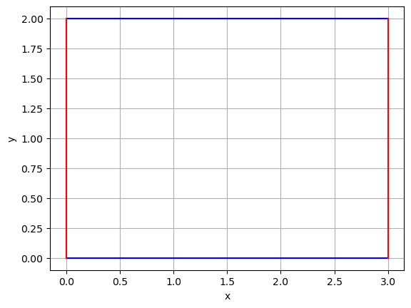
Example 5
Let
The area of the parallelogram determined by
is \(|-6| = 6\).
import matplotlib.pyplot as plt

# Define x and y values for the lines
x = range(0, 4)
y1 = [ 0 for k in x]
y2 = [ 2 for k in x]
y = range(0, 3)
x1 = [3 for k in y]
x2 = [0 for k in y]

# Plot the lines on the same plane
plt.plot(x, y1, 'b')
plt.plot(x, y2, 'b')
plt.plot(x1, y, 'r')
plt.plot(x2, y, 'r')

# Add labels to the graph
plt.xlabel('x')
plt.ylabel('y')
plt.grid()

# Show the graph
plt.show()
Example 6
Determine if the following points are coplanar.
Solution:
To determine if the above points are coplanar, we check whether or not \(det \left(\ \begin{bmatrix} 1 & 0 & 2 \\ 4 & 3 & 5 \\ 3 & 4 & 6 \end{bmatrix}\ \right) = 0\):
A = np.array([[1,0,2],[4,3,5],[3,4,6]])

det(A)
12
Since \(det(A)\neq 0\), the mentioned points are not coplanar. In fact they form a parallelepiped of volume 12.
Numerical Note#
In this section, we discussed two different ways to compute the determinant of a square matrix: cofactor expansion and row operations.
While cofactor expansion is a straightforward approach, it becomes computationally impossible for large matrices. In fact, cofactor expansion requires \(n!\) multiplications for an \(n \times n\) matrix. If a computer can perform a trillion multiplications per second, computing the determinant of a \(25 \times 25\) matrix would take approximately \(500 \times 500\) years!
On the other hand, evaluating the determinant of an \(n \times n\) matrix using row operations involves about \(\frac{2n^3}{3}\) arithmetic operations. Using this method, the determinant of a \(25 \times 25\) matrix can be computed in a fraction of a second on most microcomputers.
Exercises
Let \(A\) be an \(n\times n\) matrix such that \(A^2 = I_n\). Show that \(det(A) = \pm 1\).
Find the determinant of
using the row reduction method.
Use determinants to decide if the set
is linearly independent.
Suppose \(A\), \(B\), \(P\) are \(n\times n\) matrices, \(P\) is invertible, and \(r\) is a real number. Mark True or False:
a. \(det(A+B) = det(A) + det(B)\).
b. \(det(rA) = r \cdot det(A)\).
c. \(det(PAP^{-1}) = det(A)\).
Determine if the following points are coplanar (i.e., they lie on the same plane):