Show code cell source Hide code cell source

import numpy as np
import matplotlib.pyplot as plt
import math
%matplotlib inline

7.12. Integral Test and Income Streams

In this lab, we show that it is possible due to continuous compounding of interest to deposit a fixed amount \(P\) at time \(t=0\), and then withdraw at times \(t=1, 2, 3,...\) increasing amounts \(A+Bt\) (where \(A>0\) and \(B>0\) are constants) “in perpetuity” while always maintaining a positive balance in the account.

7.12.1. Integral Test

The integral test is one of the standard tests for convergence/divergence of an infinite series. The basic idea of the test is that for a continuous function \(f(x)\) defined on the interval \(1\le x < \infty\), the infinite series

\[\sum_{n=1}^{\infty} f(n) \]

and the improper integral

\[ \int_{x=1}^{\infty} f(x)\, dx \]

either both converge or both diverge.

7.12.2. P-Series

The integral test can be used to determine all positive values of \(p\) for which the \(p\) series

\[\sum_{n=1}^{\infty} \frac{1}{n^p} \]

converges or diverges.

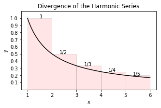
For example the case \(p=1\) so we have the harmonic series

\[\sum_{n=1}^{\infty} \frac{1}{n}. \]

The corresponding improper integral is divergent:

\[\int_{x=1}^{\infty} \frac{1}{x}\,dx = \lim_{b\rightarrow \infty} \ln x \mid _1^{b} = \lim_{b\rightarrow \infty} \ln b = \infty . \]

Thus the harmonic series is also divergent, as suggested by the circumscribed rectangles representing the first five terms in the harmonic series as shown in the figure below.

Show code cell source Hide code cell source

f = lambda x : 1/x
x=np.arange(1,6,.0001)
y=f(x)
x_left = np.arange(1,6,1)
plt.figure(figsize=(5,3))
plt.gca().set_xticks(np.arange(1,7,1))
plt.gca().set_yticks([.1,.2,.3,.4,.5,.6,.7,.8,.9,1])
plt.plot(x,y,'k',markersize=1)
plt.bar(x_left,1/x_left,width=1,alpha=0.1,align='edge',color='r',edgecolor='k')
plt.title('Divergence of the Harmonic Series')
plt.text(1.5,1,'1')
plt.text(2.3,.5,'1/2')
plt.text(3.3,.33,'1/3')
plt.text(4.3,.25,'1/4')
plt.text(5.3,.2,'1/5')
plt.xlabel('x')
plt.ylabel('y')
plt.ylim((0,1.1)) 
#plt.grid()
plt.savefig('harmonic.png')
plt.show()

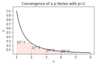
On the other hand, a \(p\)-series with \(p=2\) series must converge as shown by a convergent improper integral

\[\int_1^{\infty}\frac{1}{x^2}\,dx = \lim_{b\rightarrow\infty} -x^{-1}\mid_1^b = \lim_{b\rightarrow\infty} -\frac{1}{b}+1=1.\]

in comparison with inscribed rectangles representing the tail of the series

\[\frac{1}{2^2}+\frac{1}{3^2}+...<\int_1^{\infty}\frac{1}{x^2}=1 \Rightarrow\]

\[\sum_{n=1}^{\infty} \frac{1}{n^2}= 1+\frac{1}{2^2}+\frac{1}{3^2}+...<1+\int_1^{\infty}\frac{1}{x^2}=2.\]

Show code cell source Hide code cell source

f = lambda x : 1/x**2
x=np.arange(1,6,.0001)
y=f(x)
x_right = np.arange(2,6,1)
plt.figure(figsize=(5,3))
plt.gca().set_xticks(np.arange(1,7,1))
plt.gca().set_yticks([.1,.2,.3,.4,.5,.6,.7,.8,.9,1])
plt.plot(x,y,'k',markersize=1)
plt.bar(x_right-1,1/x_right**2,width=1,alpha=0.1,align='edge',color='r',edgecolor='k')
plt.title('Convergence of a p-Series with p=2')
plt.text(1.,.25,'1/2^2')
plt.text(2.,1/8,'1/3^2')
plt.text(3.,1/16,'1/4^2')
plt.text(4.,1/25,'1/5^2')
plt.xlabel('x')
plt.ylabel('y')
plt.ylim((0,1.1)) 
#plt.grid()
plt.savefig('p2.png')
plt.show()

7.12.3. Income Streams

If \(P\) dollars are invested into an account with interest compounded continuously with annual interest rate \(r=.05\) (i.e 5%), then after \(t\) years the amount \(P\) grows to \(Pe^{rt}=Pe^{.05t}\).

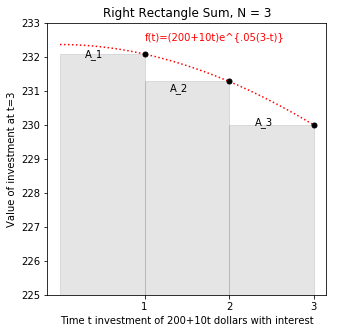
Suppose \(f(t)=200+10t\) dollars are invested into an account with the same interest rate at times \(t=1, 2, 3\) (in years) and the total including interest is computed at \(t=3\).

The amount \(\$ 210\) invested at \(t=1\) grows to \(A_1=\$ 210 e^{.05(3-1)}=210e^{.05(2).}\)

The amount \(\$ 220\) invested at \(t=2\) grows to \(A_2=\$ 220 e^{.05(3-2)}=220e^{.05(1).}\)

The amount \(\$ 230\) invested at \(t=3\) grows to \(A_3=\$ 230 e^{.05(3-3)}=230e^{.05(0)}=230.\)

Note that

\[A_1+A_2+A_3 < \int_1^3 (200+10t)e^{.05(3-t)}.\]

Show code cell source Hide code cell source

f = lambda t : (200+10*t)*math.e**(.05*(3-t))
a = 0; b = 3; N = 3
n = 10 # Use n*N+1 points to plot the function smoothly
#right endpoint rule
t = np.linspace(a,b,N+1)
y = f(t)
T = np.linspace(a,b,n*N+1)
Y = f(T)

plt.figure(figsize=(5,5))
plt.gca().set_xticks([1,2,3])
plt.plot(T,Y,'r', linestyle =':')
t_right = t[1:] # right endpoints
y_right = y[1:]
plt.plot(t_right,y_right,'k.',markersize=10)
plt.bar(t_right,y_right,width=-(b-a)/N,alpha=0.1,align='edge',color='k',edgecolor='k')
plt.title('Right Rectangle Sum, N = {}'.format(N))
plt.xlabel('Time t investment of 200+10t dollars with interest')
plt.ylabel('Value of investment at t=3')
plt.text(1,232.5,"f(t)=(200+10t)e^{.05(3-t)}",color='r')
plt.text(.3,232,"A_1")
plt.text(1.3,231,"A_2")
plt.text(2.3,230,"A_3")
plt.ylim((225, 233)) 
#plt.grid()
plt.savefig('3 period.png')
plt.show()

7.12.4. Exercises

Exercises

1. Suppose \(f(t) = 10,000+500 t\) dollars are invested into an account (with the same interest rate) at times \(t=1, 2, 3,\) and \(4\) (\(t\) in years). At time \(t=4\), find the total value of the investment with interest \(A_1+A_2+A_3+A_4.\)

2. Show geometrically that the sum \(10,500 e^{.05(3)} + 11,000 e^{.05(2)} + 11,500 e^{.05} + 12,000 \) is less than \(I_4=\int_0^4 (10,000+500 t) e^{.05 (4-t)} dt\).

3. Explain why

\[ I_4=\int_0^4 (10,000+500 t) e^{.05 (4-t)} dt = e^{.05 (4)} \int_0^4 (10,000+500 t) e^{-.05 t} dt = e^{.05(4)}P_4. \]

4. Explain why an amount \(P_4=\int_0^4 (10,000+500 t) e^{-.05 t} dt\) invested at time \(t=0\) will allow withdrawals whose total value with interest is \(A_1+A_2+A_3+A_4\).

5. Extend the reasoning in exercises 1-4 to show that \(P_N = \int_0^N (10,000+500 t) e^{-.05t } dt \) deposited at \(t=0\) is sufficient to allow \(f(t) = 10,000+500 t\) to be withdrawn from the account at \(t=1,2,...,N\). Use integration by parts to find \(P_{\infty} = \int_0^{\infty} (10,000+500 t) e^{-.05 t} dt \). (If this finite amount \(P_{\infty}\) is deposited at \(t=0\), then \(f(t)=10,000 + 500 t\) can be withdrawn at \(t=1, 2, 3,...\) (“in perpetuity”.)