Show code cell source Hide code cell source

import matplotlib.pyplot as plt
import numpy as np

7.15. JNB Lab: Calculus of Entropy in Daily Life and Monte Carlo Simulations

The goal of this lab is to explore how calculus can be used to explore the concept of entropy as might be useful within a variety of situations.

7.15.1. Derivative Optimization

Given a function \(y=f(x)\), the derivative \(f'(x)\) evaluated at \(x=a\) gives us the slope of the tangent (instantaneous rate of change) to the graph of \(y=f(x)\) and the point \((a,f(a))\). Maximum and minimum points are special since the tangents are horizontal at those points and hence the derivative satisfies the equation \(f'(x)=0\). Maximum and minimum points are important in applications since, for example, minimizing cost or maximizing the benefit of a project is often a primary goal.

Entropy is an important example discussed in the section on societal applications in the final chapter (complex systems) of this book. We illustrate here why minimization/maximization of entropy is important. Suppose you have a committee of \(N\) people voting on a certain decision such that a proportion \(p_1=p\) strongly prefers option A and a proportion \(p_2=1-p\) strongly prefers option B . Note that there is no disagreement if \(p_1=1\) and \(p_2=0\) (everyone strongly prefers option A) and likewise there is no disagreement if \(p_1=0\) and \(p_2=1\) (everyone strongly prefers option B.) Note that if \(p_1=.9\) and \(p_2=.1\), there is a strong consensus for Option A so while there is a little bit of disagreement, Option A will likely carry. Note that the case where the population is evenly split \(p_1=p_2=.5\) will have the greatest disagreement in trying to achieve a consensus.

Entropy can be used to measure the level of disagreement. We define the Shannon entropy as

\[ H(p) = -\sum_{i=1}^2 p_i \ln p_i = -[p\ln p + (1-p)\ln(1-p)]. \]

where \(0\le p \le 1\). Exercise 1.1 shows the properties of this function \(H(p)\) correspond to the amount of disagreement in our example.

Exercises

Exercises

1.1

a) Make a plot of \(H(p)= -[p\ln p + (1-p)\ln(1-p)]\) on the interval \(0<p<1\)

b) Use L’Hopital’s rule to evaluate the one-sided limits \(H(0)=\lim_{p\rightarrow 0^+} H(p)\) and \(H(1)=\lim_{p\rightarrow 1^-} H(p)\).

c) Use calculus to prove that a maximum value of \(H(p)\) occurs at \(p=.5\).

7.15.2. Series

Suppose now there are \(k\) options. \(p_i\) is the proportion of committee members favoring option \(i\) (\(1\le i \le k\) and \(p_1+....+p_k=1\)).

\[ H= -\sum_{i=1}^k p_i \ln p_i= -(p_1\ln p_1 + p_2\ln p_2 + ... + p_k \ln p_k). \]

Exercises

Exercises

2.1

1. Consider the case with \(k=3\). Compute the entropy \(H\) if

   a) \(p_1=.5, p_2=.3, p_3=.2\) and

   b) \(p_1=.2, p_2=.5, p_3=.3\)

   c) \(p_1=.2, p_2=.3, p_3=.5\)

2. What does problem 1 tell us about the computation of entropy of disagreement?

7.15.3. Probability Distributions

Now let us consider a situation where you are holding a dinner and there is a certain probability \(p_k\) that a guest prefers to arrive between \(k\) and \(k+1\) hours late. If all guests prefer to arrive no more than 1/2 hour late, then \(p_0=1\) and all other \(p_k=0\), so the entropy \(H=0\). This is in certain cultures an ideal situation and there is no major disagreement in the preferred arrival time (\(H=0\)).

In other cases, it might be normative for guests to arrive substantially later than the announced time. For example, if all guests prefer to arrive between \(k=1\) and \(k=2\) (between 1 and 2 hours late), then \(p_1=1\) and again there is no major disagreement (\(H=0\)).

We can use a probability distribution to model the probability of a preferred arrival time. For example, if the mean arrival time is 10 minutes after the designated time (1/k=1/6 hour), then we consider the probability density function \(f(x)=\frac{1}{6} e^{-6x}\) where \(x\in[0,\infty)\). The probability that a guest arrives in the interval \(k\le x \le k+1\) is given by the definite integral

\[ p_k=prob(k\le x \le k+1) = \int_k^{k+1} f(x)\, dx = (1/6) \int_k^{k+1} e^{-6x}\,dx= -\frac{1}{36} e^{-6x} \mid_k^{k+1} = -\frac{1}{36}[e^{-6(k+1)}-e^{-6k}]. \]

For example, \(p_0= - \frac{1}{36}[ e^{-6} -1] \approx .9999 \)

and

\(p_1=- \frac{1}{36}[ e^{-6(2)} -exp(-6)] \approx .0001\)

so

\(H\approx .001\). (There is almost no disagreement in preferred arrival time.)

7.15.4. Exercises

Exercises

3.1 An exponential distribution has the form \(f(x)=ke^{-kx}\) where \(k>0\) and \(0\le x < \infty\).

a) Show that \(prob(0\le x < \infty) = 1\).

b) Given a continuous probability distribution \(f(x)\) for \(x\in I\), the mean is computed as \(\int_{x\in I} x f(x)\, dx\). Find the mean for the exponential distribution in terms of \(k\)

7.15.5. Monte Carlo Simulation

Let us consider the context of teaching a class of math students with a random variable \(X\) denoting a standardized entrance test score. If \(X<0\), the score is below average, and if \(X>0\) , the score is above average. Note that if all students are average, teaching the class is simpler than if there is a big spread in the students’ range of ability. Entropy in this case is interpreted in this case to mean complexity.

Here we would like to compare two distributions with domain \(-\infty < x < \infty\):

\(f(x) = \frac{1}{\sqrt{2\pi}} e^{-x^2}\) (standard unit normal distribution)

\(g(x) = \frac{1}{\pi} \frac{1}{1+x^2}\) (Cauchy distribution)

In particular, we would like to compare the contribution to the complexity (entropy) for the tails \(x<-3\) and \(x>3\). We will classify students as ‘usual’ if \(-3\le X \le 3\) and `exceptional’ if \(x>3\) or \(X<-3\).

In practical terms, we are asking how the complexity is impacted by very strong or very weak students for these two distributions.

Intuitively we know for a normal distribution, there is only a .3% chance of being more than 3 standard deviations above or below the mean. So for a class, say of 10 students, we would expect .03 students to be exceptional. So there would be essentially no contribution to the complexity from a perspective focused on tangible results.

On the other hand, for a Cauchy distribution the probability is .2 to get a very strong or a very weak student, and so for a class of 10 students, we would expect to see 2 exceptional students. The contribution to complexity is \(H_{tail} = -.2 ln (.2)\approx .1\).

To estimate the complexity of a normally distributed vs. Cauchy distributed class, we can use a Monte Carlo simulation. That is, we draw a sample of 10 random values, determine the proportion of usual and exceptional students, and compute the entropy. We illustrate this for a routine class (normally distributed) and ask you to analyze a Cauchy distributed class.

Show code cell source Hide code cell source

trials=10000
class_size=10
s = np.random.standard_normal(trials*class_size)

Hroutine=[]
Hexceptional=[]
Hsum=[]
k=0

for j in np.arange(0,trials,1):
    routine=0
    exceptional=0
    for i in np.arange(0,10,1):   
        if s[k]>3 or s[k]<-3:
            exceptional=exceptional+1
            k=k+1
        else: 
            routine=routine+1
            k=k+1
    if routine>0:
        p=routine/10
        Hroutine.append(-p*np.log(p))
    else:
        Hroutine.append(0)
    if exceptional>0:
        p=exceptional/10
        Hexceptional.append(-p*np.log(p))
    else:
        Hexceptional.append(0)
    Hsum.append(Hroutine[j]+Hexceptional[j])
        
H=np.mean(Hsum)
Hex=np.mean(Hexceptional)

print("Entropy of Normal Class=", H)  
print("Contribution to Entropy by Exceptional Students=", Hex)

Entropy of Normal Class= 0.008372164361174893
Contribution to Entropy by Exceptional Students= 0.005926806596313439

Exercises

Exercises

4.1

a) Sketch the unit normal and Cauchy distributions on the interval \(-5\le x \le 5\). What do you note about the tails of these distributions?

b) Do a Monte Carlo simulation with 10,000 trials to estimate the entropy of a Cauchy distributed class with 10 students as well as the contribution to the entropy by exceptional students.

7.15.6. Random Number Simulation of a Drive-thru

The goal of this lab is to show how random numbers are used to simulate a scenario where the owner of a fast-food restaurant is contemplating whether or not to open a second drive-thru lane as illustrated in the animation below. (For an explanation of how to create this animation, see the section on object-oriented programming in the chapter Overview of Python Programming.) The section on Chicago homicides gives a related example of how random numbers can be used in “Monte Carlo simulation”.

Our main reference for this modeling problem is described in the video by Daniel Hickman below:

Link

7.15.7. Model Distributions

A drive-thru model begins with empirical data which can be described using probability density functions (PDFs), also called distributions. We use the same distributions given in Hickman’s video as summarized below:

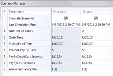
We will explain a value \(r\) generated by a PRNG (pseudo-random number generator) can be converted into

• A=length of time before the next car arrives at the parking lot

• O=length of time to place an order

• P=length of time to pay for the food

• F=length of time to pick up food

A=Length of time before next arrival

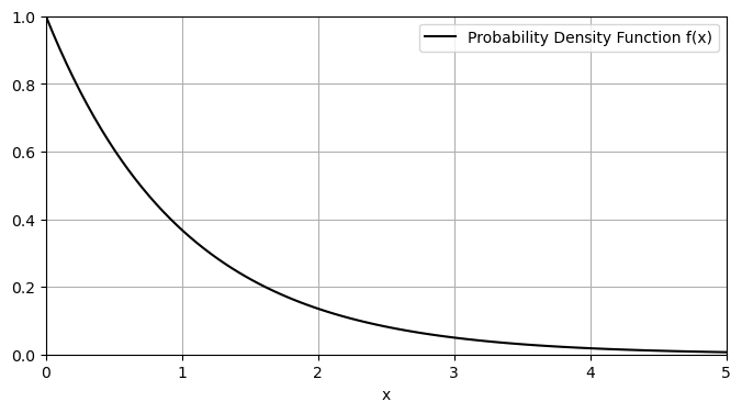
Let \(X\) be a random variable giving the length of time (in minutes) until the next car arrives at the parking lot. We assume \(X\) is an exponential distribution with mean \(1/k=1\). In this case, the probability density function (pdf) is

\[ f(x)=ke^{-kx}=e^{-x} \]

Here is a graph of this pdf:

import numpy as np
import matplotlib.pyplot as plt
x = np.linspace(0,5,100)
f= np.exp(-x)  #standard (unit) normal distribution
plt.figure(figsize=(8, 4))
plt.plot(x,f,color='k',label="Probability Density Function f(x)")
plt.xlim((0,5))
plt.ylim((0,1))
plt.xlabel("x")
plt.grid()
plt.legend()
plt.show()

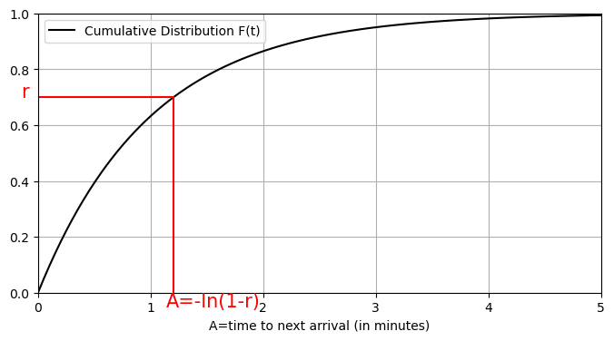
The corresponding cumulative distribution function (cdf) is

\[ F(t) = prob(0\le X \le t) = \int_0^t k e^{-kx}\,dx = - e^{-kx}\mid_0^t= -e^{-kt}+1=-e^{-t}+1. \]

Here is a graph of this cdf:

import numpy as np
import matplotlib.pyplot as plt
t = np.linspace(0,5,100)
F= 1-np.exp(-t)  #standard (unit) normal distribution
plt.figure(figsize=(8, 4))
plt.plot(t,F,color='k',label="Cumulative Distribution F(t)")
plt.xlim((0,5))
plt.ylim((0,1))
plt.xlabel("A=time to next arrival (in minutes)")
plt.grid()
plt.legend()
plt.show()

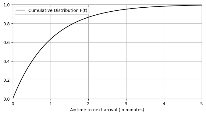
Note that the \(F(t)=1-e^{-t}\) is an increasing function with a value of 0 at \(t=0\) and a range \([0,1)\). As such, each random number \(r\) \((0\le r <1)\) corresponds to a unique value of \(A\):

\[ r=1-e^{-kA}\,\, \Rightarrow \]

\[ e^{-kA}=1-r\,\, \Rightarrow \]

\[ -kA = \ln (1-r) \,\,\Rightarrow \]

\[ A=-\frac{1}{k}\ln(1-r)=-\ln(1-r). \]

import numpy as np
import matplotlib.pyplot as plt
t = np.linspace(0,5,100)
F= 1-np.exp(-t)  #standard (unit) normal distribution
plt.figure(figsize=(8, 4))
plt.plot(t,F,color='k',label="Cumulative Distribution F(t)")
plt.xlim((0,5))
plt.ylim((0,1))
plt.text(-.15,.7,"r",color='r',size=15)
plt.text(-np.log(1-.7)-.07,-.05,"A=-ln(1-r)",color='r',size=15)
plt.plot([0,-np.log(.3),-np.log(.3)],[.7,.7,0],color='r')
plt.xlabel("A=time to next arrival (in minutes)")
plt.grid()
plt.legend()
plt.show()

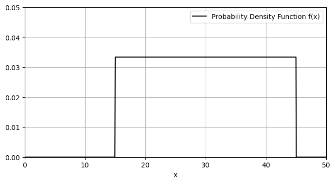
O=length of time to place an order

Let \(X\) be a random variable giving the length of time (in seconds) to place an order. We assume \(X\) is uniformly distributed on the interval [15,45] (denoted U(30,15) where 30 is the length of the interval and 15 is the minimum value for \(X\).) In this case, the probability density function (pdf) is

\[ f(x)=\frac{1}{30}\,\,(15\le x \le 45) \]

import numpy as np
import matplotlib.pyplot as plt
x = np.linspace(0,50,1000)
f= (1/30)*(np.heaviside(x-15,0)-np.heaviside(x-45,0))   #standard (unit) normal distribution
plt.figure(figsize=(8, 4))
plt.plot(x,f,color='k',label="Probability Density Function f(x)")
plt.xlim((0,50))
plt.ylim((0,.05))
plt.xlabel("x")
plt.grid()
plt.legend()
plt.show()

The cumulative distribution function (cdf) is

\[ F(t) = prob(15\le X \le t) = \int_0^t \frac{1}{30}\,dx = - \frac{1}{30}x\mid_{15}^t= \frac{t}{30}-\frac{15}{30}=\frac{t-15}{30} \]

Here is a graph of this cdf:

import numpy as np
import matplotlib.pyplot as plt
t = np.linspace(15,45,100)
F= ((t-15)/30)*np.heaviside(t-15,0)  #U(30,15)
plt.figure(figsize=(8, 4))
plt.plot(t,F,color='k',label="Cumulative Distribution F(t)")
plt.xlim((15,45))
plt.ylim((0,1))
plt.xlabel("O=time to place order (in seconds)")
plt.grid()
plt.legend()
plt.show()

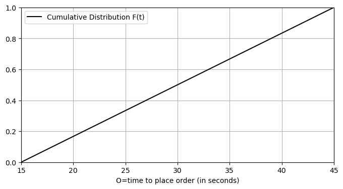
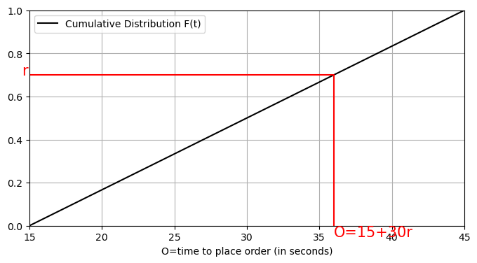
As before, the \(F(t)=\frac{t-15}{30}\) \(\,(15 \le t \le 45\)) is an increasing function with a value of 0 at \(t=15\) and a range \([0,1)\).

As such, each random number \(r\) \((0\le r <1)\) corresponds to a unique value of \(O\) where \(\,15 \le O\le 45\):

\[ r=\frac{O-15}{30}\,\, \Rightarrow \]

\[ O-15=30r\,\, \Rightarrow \]

\[ O=15+30r. \]

import numpy as np
import matplotlib.pyplot as plt
t = np.linspace(15,45,100)
F= ((t-15)/30)*np.heaviside(t-15,0) # U(30,15)
plt.figure(figsize=(8, 4))
plt.plot(t,F,color='k',label="Cumulative Distribution F(t)")
plt.xlim((15,45))
plt.ylim((0,1))
plt.text(15-.5,.7,"r",color='r',size=15)
plt.text(15+30*.7,-.05,"O=15+30r",color='r',size=15)
plt.plot([15,15+30*.7,15+30*.7],[.7,.7,0],color='r')
plt.xlabel("O=time to place order (in seconds)")
plt.grid()
plt.legend()
plt.show()

Similarly, we can convert a random number \(r\) into a length of time \(P\) to pay for food or a length of time \(F\) to pick up food.

P=length of time to pay for the food

By Cash

Let \(X\) be a random variable giving the length of time (in seconds) to pay for an order using cash. We assume \(X\) is uniformly distributed on the interval [5,35] (denoted U(30,5) where 30 is the length of the interval and 5 is the minimum value for \(X\) in seconds.) In this case, the probability density function (pdf) is

\[ f(x)=\frac{1}{30}\,\,(5\le x \le 35) \]

The cdf is

\[ F(t)=\frac{1}{30}(t-5) \]

($5\le t\le 35).

Given a random number \(r\) (\(0\le r \le 1\)), the pay by cash time is \(P=30r+5\).

By Credit

Let \(X\) be a random variable giving the length of time (in seconds) to pay for an order using a credit card. We assume \(X\) is uniformly distributed on the interval [5,20] (denoted U(15,5) where 15 is the length of the interval and 5 is the minimum value for \(X\) in seconds.) In this case, the probability density function (pdf) is

\[ f(x)=\frac{1}{15}\,\,(5\le x \le 20) \]

The cdf is

\[ F(t)=\frac{1}{15}(t-5) \]

(\(5\le t\le 20\)).

Given a random number \(r\) (\(0\le r \le 1\)), the pay by cash time is \(P=15r+5\).

F=length of time to pick up food

Let \(X\) be a random variable giving the length of time (in seconds) to pick up an order. We assume \(X\) is uniformly distributed on the interval [30,90] (denoted U(60,30) where 60 is the length of the interval and 30 is the minimum value for \(X\) in seconds.) In this case, the probability density function (pdf) is

\[ f(x)=\frac{1}{60}\,\,(30\le x \le 90) \]

The cdf is

\[ F(t)=\frac{1}{60}(t-30) \]

\[ ($30\le t\le 90). \]

Given a random number \(r\) (\(0\le r \le 1\)), the pay by cash time is \(P=60r+30\).

Exercises

5.1

a) Use random numbers to simulate arrivals at a one-lane drive-thru. For simplicity, assume that:

the time \(A\) between arrivals is exponentially distributed with mean \(k\)=1 (in minutes);

the order time \(O\) is uniformly distributed on the interval \([15,45]\) (in seconds);

the pay time \(P\) is unformly distributed on the interval \([5,25]\) (in seconds); and

the food pick-up time \(F\) is uniformly distributed on the interval \([30,60]\) in seconds.

Find the mean total time to enter and be processed through the order-pay-pickup system.

Be sure to convert the time between arrivals to seconds and give the final mean total time in minutes.

b) Explore how the mean total time depends on system parameters. For example, you might vary the parameter \(k\) in the arrival time from k=.1 (6 seconds) to 2 (2 minutes) in increments of .1