11.5. Systems of First-Order Differential Equations

Note

This chapter offers an exploration into an essential component of the mathematical toolkit, used across numerous scientific and engineering disciplines. As we already know, differential equations are mathematical statements that describe the rates at which quantities change. However, reality often presents us with scenarios where multiple interrelated quantities are changing simultaneously. Enter the realm of systems of differential equations, a powerful extension of single differential equations, allowing us to model and understand a multitude of complex phenomena.

In this chapter, we specifically focus on systems of first-order differential equations. First-order means that only the first derivative of the function(s) appears in the system, but this doesn’t imply simplicity. Even with this limitation, these systems can model a wide array of phenomena, from predator-prey relationships in ecology to interconnected circuits in electronics, oscillating chemical reactions, and the spread of diseases in populations, among many others.

11.5.1. Introduction to Systems of Linear Differential Equations

A system of first-order differential equations in \(n\) unknown functions \(x_1(t), x_2(t), \dots, x_n(t)\) is a collection of \(n\) differential equations with \(n\) dependent variables. That is,

\[\dfrac{dx_1}{dt} = f_1(t, x_1, x_2, \dots, x_n)\]

\[\dfrac{dx_2}{dt} = f_2(t, x_1, x_2, \dots, x_n)\]

\[\vdots\]

\[\dfrac{dx_n}{dt} = f_n(t, x_1, x_2, \dots, x_n).\]

In this case, a solution is a collection of \(n\) functions satisfying all of these equations. We should also note that every order \(n\) differential equation can be written as a system of \(n\) first-order differential equations.

Example

Write the differential equation \(x'''+4x''+2x'+x=t^2+\cos(t)\) as a system of three first-order differential equations.

First we will define new variables. Let \(x_1 = x, x_2=x', x_3 = x''\). Then

\[x'''+4x''+2x'+x= x_3'+4x_3+2x_2+x_1 = t^2+\cos(t).\]

Rewriting this as a system yields

\[x_1' = x_2\]

\[x_2' = x_3\]

\[x_3' = -x_1-2x_2-4x_3+t^2+\cos(t)\]

Example

Find a system of first-order differential equations which are equivalent to the system

\[x'' = x+y\cos(t)\]

\[y'' = x\ln(t)+y'.\]

First we will define new variables. Let \(x_1 = x, x_2=x', y_1 = y, y_2 = y'\).

Rewriting this as a system yields

\[x_1' = x_2\]

\[x_2' = x_1+y_1\cos(t)\]

\[y_1' = y_2\]

\[y_2' = x_1\ln(t)+y_2\]

A system of linear first-order differential equations (or simply linear system in \(n\) unknown functions \(x_1(t), x_2(t), \dots, x_n(t)\)) is a system of the form

\[x_1' = a_{11}(t)x_1 + a_{12}(t)x_2 + \dots + a_{1n}(t)x_n + b_1(t)\]

\[x_2' = a_{21}(t)x_1 + a_{22}(t)x_2 + \dots + a_{2n}(t)x_n + b_2(t)\]

\[\vdots\]

\[x_n' = a_{n1}(t)x_1 + a_{n2}(t)x_2 + \dots + a_{nn}(t)x_n + b_n(t)\]

where \(a_{ij}(t)\) and \(b_i(t)\) are arbitrary functions in the independent variable \(t\). If \(b_i(t)=0\) for all \(1 \leq i \leq n\), we say that the linear system is homogeneous. The number of dependent variables of the linear system is called the dimension of the system.

11.5.2. Solving Homogeneous Linear Systems with Constant Coefficients

The set \(\{v_1(t), v_2(t), \dots, v_n(t)\}\) where \(v_i(t) = \begin{bmatrix} v_{i1}(t) \\ v_{i2}(t) \\ \vdots \\ v_{in}(t) \end{bmatrix}\) is called linearly dependent if there exist scalars \(c_1, c_2, \dots, c_n \in \mathbb{R}\), at least one of which is not zero, such that

\[c_1v_1(t) + c_2v_2(t) + \dots + c_nv_n(t) = 0.\]

If no such scalars exist, the set of vector functions is linearly independent.

Note: We saw the same notion for functions and vectors when looking at solving linear (usually second order) homogeneous differential equations with constant coefficients.

Example

• \(\biggl\{\begin{bmatrix} e^{2t} \\ e^{3t} \end{bmatrix}, \begin{bmatrix} e^{3t} \\ e^{2t} \end{bmatrix}\biggr\}\) are linearly independent.

• \(\biggl\{\begin{bmatrix} e^{2t} \\ e^{3t} \end{bmatrix}, \begin{bmatrix} 4e^{2t} \\ 4e^{3t} \end{bmatrix}\biggr\}\) are linearly dependent as \(4\begin{bmatrix} e^{2t} \\ e^{3t} \end{bmatrix} - \begin{bmatrix} 4e^{2t} \\ 4e^{3t} \end{bmatrix} = \begin{bmatrix} 0 \\ 0 \end{bmatrix}\)

• \(\biggl\{v_1(t) = \begin{bmatrix} \sin(t) \\ t \end{bmatrix}, v_2(t)= \begin{bmatrix} \sin(t) \\ 3t \end{bmatrix}, v_3(t) = \begin{bmatrix} 0 \\ -2t \end{bmatrix}\biggr\}\) are linearly dependent as \(v_1(t)-v_2(t)-v_3(t) =\vec{0}\).

If \(x' = Ax\) is a homogeneous linear system of first-order differential equations with \(n \times n\) coefficient matrix \(A\), any set of \(n\) linearly independent vector solutions to the system on a given interval \(I\) is called a fundamental set of solutions to the system. If \(\{v_1(t), v_2(t), \dots, v_n(t)\}\) is a fundamental set of solutions, then

\[x(t) = c_1v_1(t) + c_2v_2(t) + \dots + c_nv_n(t)\]

is called the general solution.

Example

Consider the system

\[\begin{split} x' = \begin{bmatrix} 5 & -4 \\ 2 & -1 \end{bmatrix}x. \end{split}\]

Verify that

\[\begin{split} \biggl\{ \begin{bmatrix} 2e^{3t} \\ e^{3t} \end{bmatrix}, \begin{bmatrix} e^t \\ e^t \end{bmatrix} \biggr\} \end{split}\]

forms a fundamental solution set.

Step 1: Substituting in both vectors from the fundamental solution set to the left hand side yields

\[\begin{split} \frac{d}{dt}\left( \begin{bmatrix} 2e^{3t} \\ e^{3t} \end{bmatrix}\right) = \begin{bmatrix} 6e^{3t} \\ 3^{3t} \end{bmatrix} \end{split}\]

and

\[\begin{split} \frac{d}{dt}\left( \begin{bmatrix} e^t \\ e^t \end{bmatrix}\right) = \begin{bmatrix} e^t \\ e^t \end{bmatrix}. \end{split}\]

Step 2: Substituting in both vectors from the fundamental solution set to the right hand side yields

\[\begin{split} \begin{bmatrix} 5 & -4 \\ 2 & -1 \end{bmatrix}\begin{bmatrix} 2e^{3t} \\ e^{3t} \end{bmatrix} = \begin{bmatrix} 10e^{3t}-4e^{3t} \\ 4e^{3t}-e^{3t} \end{bmatrix} = \begin{bmatrix} 6e^{3t} \\ 3e^{3t} \end{bmatrix} \end{split}\]

and

\[\begin{split} \begin{bmatrix} 5 & -4 \\ 2 & -1 \end{bmatrix}\begin{bmatrix} e^{t} \\ e^{3t} \end{bmatrix} = \begin{bmatrix} 5e^{t}-4e^{t} \\ 2e^{t}-e^{t} \end{bmatrix} = \begin{bmatrix} e^{t} \\ e^{t} \end{bmatrix}, \end{split}\]

Step 3: Notice that both vectors are solutions to the system. Now to verify that they form a fundamental set of solutions, we simply need to check that the two vectors are linearly independent. Solving the system

\[ 2c_1e^{3t}+c_2e^t = 0 \]

\[ c_1e^{3t}+c_2e^t =0 \]

gives that \(c_1=c_2=0\). Thus the vectors are linearly independent.

This means the general solution to this system is

\[\begin{split} x(t) = c_1\begin{bmatrix} 2 \\ 1 \end{bmatrix}e^{3t} + c_2\begin{bmatrix} 1 \\ 1 \end{bmatrix}e^{t}. \end{split}\]

Natural Question

Where do the functions \(e^t\) and \(e^{3t}\) and the vectors \(\begin{bmatrix} 2 \\ 1 \end{bmatrix}\) and \(\begin{bmatrix} 1 \\ 1 \end{bmatrix}\) come from?

It turns out that these values come from the eigenvalues and eigenvectors of \(\begin{bmatrix} 5 & -4 \\ 2 & -1 \end{bmatrix}\). So let’s compute those values!

\[\det(A_\lambda I) = 0\]

\[\begin{split}\det\left(\begin{bmatrix} 5-\lambda & -4 \\ 2 & -1-\lambda \end{bmatrix} \right)=0\end{split}\]

\[(5 - \lambda)(-1-\lambda)-(-8)=0\]

\[\lambda^2-4\lambda+3=0\]

\[(\lambda-3)(\lambda-1)=0\]

Thus the eigenvalues are \(\lambda=1\) and \(\lambda=3\).

Now we want to find the eigenvectors associated to each eigenvalue. Let’s start with \(\lambda =1\).

Setting up the augmented matrix yields

\[\begin{split}\left[ \begin{matrix} 5-1 & -4 \\ 2 & -1-1 \\ \end{matrix} \left| \, \begin{matrix} 0 \\ 0 \\ \end{matrix} \right. \right] = \left[ \begin{matrix} 4 & -4 \\ 2 & -2 \\ \end{matrix} \left| \, \begin{matrix} 0 \\ 0 \\ \end{matrix} \right. \right] \approx \left[ \begin{matrix} 1 & -1 \\ 0 & 0 \\ \end{matrix} \left| \, \begin{matrix} 0 \\ 0 \\ \end{matrix} \right. \right]\end{split}\]

Thus an eigenvector associated to \(\lambda=1\) is \(\begin{bmatrix} 1 \\ 1 \end{bmatrix}\).

Let’s now consider \(\lambda = 3\).

Setting up the augmented matrix yields

\[\begin{split}\left[ \begin{matrix} 2 & -4 \\ 2 & -4 \\ \end{matrix} \left| \, \begin{matrix} 0 \\ 0 \\ \end{matrix} \right. \right] \approx \left[ \begin{matrix} 1 & -2 \\ 0 & 0 \\ \end{matrix} \left| \, \begin{matrix} 0 \\ 0 \\ \end{matrix} \right. \right]\end{split}\]

Thus an eigenvector associated to \(\lambda=3\) is \(\begin{bmatrix} 2 \\ 1 \end{bmatrix}\).

Notice that these values recover the information from the fundamental solution set in the previous example.

Theorem

Let \(A\) be an \(n \times n\) matrix of real numbers with \(n\) distinct real eigenvalues \(\lambda_1, \lambda_2, \dots, \lambda_n\) with respective eigenvectors \(v_1, v_2, \dots, v_n\). Then

\[\{v_1e^{\lambda_1 t}, v_2e^{\lambda_2 t}, \dots, v_ne^{\lambda_n t}\}\]

is a fundamental set of solutions to the homogeneous linear system \(x' = Ax\).

Example

Solve the initial-value problem

\[\begin{split}x' = \begin{bmatrix} 5 & 3 \\ 6 & 2 \end{bmatrix}x, \quad x(0) = \begin{bmatrix} 0 \\ 3 \end{bmatrix}.\end{split}\]

\[\det(A-\lambda I) = 0\]

\[\begin{split}\det\left(\begin{bmatrix} 5-\lambda & 3 \\ 6 & 2-\lambda \end{bmatrix} \right)=0\end{split}\]

\[(5 - \lambda)(2-\lambda)-(18)=0\]

\[\lambda^2-7\lambda-8=0\]

\[(\lambda+1)(\lambda-8)=0\]

Thus the eigenvalues are \(\lambda=-1\) and \(\lambda=8\).

Now we want to find the eigenvectors associated to each eigenvalue. Let’s start with \(\lambda =-1\).

Setting up the augmented matrix yields

\[\begin{split} \left[ \begin{matrix} 5-(-1) & 3 \\ 6 & 2-(-1) \\ \end{matrix} \left| \, \begin{matrix} 0 \\ 0 \\ \end{matrix} \right. \right] = \left[ \begin{matrix} 6 & 3 \\ 6 & 3 \\ \end{matrix} \left| \, \begin{matrix} 0 \\ 0 \\ \end{matrix} \right. \right] \approx \left[ \begin{matrix} 1 & \frac{1}{2} \\ 0 & 0 \\ \end{matrix} \left| \, \begin{matrix} 0 \\ 0 \\ \end{matrix} \right. \right] \end{split}\]

Thus an eigenvector associated to \(\lambda=-1\) is \(\begin{bmatrix} \frac{-1}{2} \\ 1 \end{bmatrix}\).

Let’s now consider \(\lambda = 8\).

Setting up the augmented matrix yields

\[\begin{split} \left[ \begin{matrix} -3 & 3 \\ 6 & -6 \\ \end{matrix} \left| \, \begin{matrix} 0 \\ 0 \\ \end{matrix} \right. \right] \approx \left[ \begin{matrix} 1 & -1 \\ 0 & 0 \\ \end{matrix} \left| \, \begin{matrix} 0 \\ 0 \\ \end{matrix} \right. \right] \end{split}\]

Thus an eigenvector associated to \(\lambda=8\) is \(\begin{bmatrix} 1 \\ 1 \end{bmatrix}\).

This means the general solution to this system is \(x(t) = c_1\begin{bmatrix} \frac{-1}{2} \\ 1 \end{bmatrix}e^{-t} + c_2\begin{bmatrix} 1 \\ 1 \end{bmatrix}e^{8t}\).

Using the initial condition, we find that

\[\begin{split}\begin{bmatrix} 0 \\ 3 \end{bmatrix} = c_1\begin{bmatrix} \frac{-1}{2} \\ 1 \end{bmatrix}e^{-(0)} + c_2\begin{bmatrix} 1 \\ 1 \end{bmatrix}e^{8(0)}\end{split}\]

\[\begin{split}\begin{bmatrix} 0 \\ 3 \end{bmatrix} = c_1\begin{bmatrix} \frac{-1}{2} \\ 1 \end{bmatrix} + c_2\begin{bmatrix} 1 \\ 1 \end{bmatrix}\end{split}\]

This is equivalent to solving

\[0 = \frac{-1}{2}c_1 + c_2\]

\[3 = c_1+c_2.\]

Solving this system for \(c_1\) and \(c_2\) gives \(c_1=2\) and \(c_2=1\).

Thus the solution to the initial value problem is

\[\begin{split}x(t) = 2\begin{bmatrix} \frac{-1}{2} \\ 1 \end{bmatrix}e^{-t} + \begin{bmatrix} 1 \\ 1 \end{bmatrix}e^{8t}.\end{split}\]

Now let’s consider what happens when we do not have \(n\) distinct eigenvalues. In other words, what happens when an eigenvalue occurs with some multiplicity.

Motivating Example

Consider the following matrices

\[\begin{split} B = \begin{bmatrix} 2 & 0 & 0 \\ 0 & 1 & 1 \\ 0 & 1 & 1 \end{bmatrix} \quad \quad C=\begin{bmatrix} 3 & 1 \\ -1 & 1 \end{bmatrix}.\end{split}\]

Both of these matrices have \(\lambda=2\) as an eigenvalue with multiplicity 2.

In the case of matrix \(B\), \(\lambda=2\) has two linearly independent eigenvectors \(\begin{bmatrix} 1 \\ 0 \\ 0 \end{bmatrix}\) and \(\begin{bmatrix} 0 \\ 1 \\ 1 \end{bmatrix}.\) In this case, the procedure for finding the general solution to the equation \(x'=Bx\) has not changed from the previous examples.

However, in the case of matrix \(C\), \(\lambda=2\) has only one eigenvector \(\begin{bmatrix} -1 \\ 1\end{bmatrix}\) despite having multiplicity 2. In this case, the procedure for finding the general solution to the equation \(x'=Cx\) will need to be changed as we do not have enough linearly independent pieces for our fundamental solution set.

Let \(A\) be an \(n \times n\) matrix with eigenvalue \(\lambda\) appearing with multiplicity \(k\) in the characteristic polynomial. The eigenvalue \(\lambda\) has at least 1 and at most \(k\) linearly independent eigenvectors. The eigenvalue \(\lambda\) is called defective if there are fewer than \(k\) linearly independent eigenvectors.

There are a few significant observations we should make about this example and subsequent definition. First, if a matrix has \(n\) distinct eigenvalues, none of the eigenvalues will be defective. Second, if \(\lambda\) is not defective, then the initial procedure we establish for distint real eigenvalues will still work. Finally, if \(\lambda\) is defective, we will need to produce at least one (if not more) additional solution to create the full fundamental solution set.

Example

Solve the linear system of differential equations

\[\begin{split}x' = \begin{bmatrix} 3 & 1 \\ -1 & 1 \end{bmatrix}x.\end{split}\]

\[\det(C-\lambda I) = 0\]

\[\begin{split}\det\left(\begin{bmatrix} 3-\lambda & 1 \\ -1 & 1-\lambda \end{bmatrix} \right)=0\end{split}\]

\[(3 - \lambda)(1-\lambda)-(-1)=0\]

\[\lambda^2-4\lambda+4=0\]

\[(\lambda-2)^2=0\]

Thus the eigenvalue is \(\lambda=2\) with multiplicity 2.

Now we want to find the eigenvector(s) associated with \(\lambda=2\).

Setting up the augmented matrix yields

\[\begin{split} \left[ \begin{matrix} 3-(2) & 1 \\ -1 & 1-(2) \\ \end{matrix} \left| \, \begin{matrix} 0 \\ 0 \\ \end{matrix} \right. \right] = \left[ \begin{matrix} 1 & 1 \\ -1 & -1 \\ \end{matrix} \left| \, \begin{matrix} 0 \\ 0 \\ \end{matrix} \right. \right] \approx \left[ \begin{matrix} 1 & 1 \\ 0 & 0 \\ \end{matrix} \left| \, \begin{matrix} 0 \\ 0 \\ \end{matrix} \right. \right] \end{split}\]

Thus the eigenvector associated to \(\lambda=2\) is \(\begin{bmatrix} -1 \\ 1 \end{bmatrix}\).

Let’s now guess another solution. The guess is \(\begin{bmatrix} -1 \\ 1 \end{bmatrix} te^{2t}\).

Notice

\[\begin{split} C\begin{bmatrix} -1 \\ 1 \end{bmatrix} te^{2t} = \begin{bmatrix} 3 & 1 \\ -1 & 1 \end{bmatrix} \begin{bmatrix} -1 \\ 1 \end{bmatrix} te^{2t} = \begin{bmatrix} -2 \\ 2 \end{bmatrix} te^{2t} \end{split}\]

and

\[\begin{split} \frac{d}{dt}\left( \begin{bmatrix} -1 \\ 1 \end{bmatrix} te^{2t} \right) = \begin{bmatrix} -1 \\ 1 \end{bmatrix}e^{2t}+ \begin{bmatrix} -2 \\ 2 \end{bmatrix} te^{2t}. \end{split}\]

Notice these are not quite equal, but they are close!

Let’s make a new guess. The guess is \(\begin{bmatrix} -1 \\ 1 \end{bmatrix} te^{2t}+ \begin{bmatrix} w_1 \\ w_2 \end{bmatrix} e^{2t}\) where \(\begin{bmatrix} 3-2 & 1 \\ -1 & 1-2 \end{bmatrix} \begin{bmatrix} w_1 \\ w_2 \end{bmatrix} =\begin{bmatrix} -1 \\ 1 \end{bmatrix} \). We can verify that this new guess is in fact a solution!

This means the general solution to this system is \(x(t) = c_1\begin{bmatrix} -1 \\ 1 \end{bmatrix}e^{2t} + c_2\left(\begin{bmatrix} -1 \\ 1 \end{bmatrix}te^{2t}+ \begin{bmatrix} -2 \\ 1 \end{bmatrix} e^{2t} \right)\).

Theorem

If \(x'=Ax\) is a homogeneous linear system and \(\lambda\) is a defective eigenvalue of multiplicity 2 with corresponding eigenvalue \(v\), then

\[vte^{\lambda t} + we^{\lambda t}\]

where \(w\) is any solution to

\[(A- \lambda I)w = v\]

is another solution to \(x'=Ax\). Moreover, this solution is linearly independent to the other solution associated with \(\lambda\) by construction.

Now let’s consider what happens when we have complex eigenvalues. It turns out that in this case, we have a nice procedure we can follow. Suppose \(A\) has eigenvalues \(\lambda = a \pm bi\). Then we can produce real valued solutions to \(x' = Ax\) associated to these eigenvalues as follows:

1. Choose one of the eigenvalues \(\lambda = a \pm bi\).

2. Find an eigenvector \(v\) associated to \(\lambda\).

3. Rewrite the solution \(x(t) = ve^{\lambda t} = \text{ Re}(x(t))+i\text{Im}(x(t))\) using Euler’s formula and algebra.

4. \(\text{Re}(x(t))\) and \(\text{Im}(x(t))\) are real-valued solutions to the linear system of differential equations so we can add them to the fundamental solution set.

Now let’s see this procedure applied to an example.

Example

Solve the linear system of differential equations

\[\begin{split}x' = \begin{bmatrix} 4 & -10 \\ 2 & -4 \end{bmatrix}x.\end{split}\]

\[\det(A-\lambda I) = 0\]

\[\begin{split}\det\left(\begin{bmatrix} 4-\lambda & -10 \\ 2 & -4-\lambda \end{bmatrix} \right)=0\end{split}\]

\[(4 - \lambda)(-4-\lambda)+(20)=0\]

\[\lambda^2+4=0\]

Thus the eigenvalues are \(\lambda=\pm 2i\).

Now we want to find the eigenvector associated with \(\lambda=-2i\).

Setting up the augmented matrix yields

\[\begin{split} \left[ \begin{matrix} 4-(-2i) & -10 \\ 2 & -4-(-2i) \\ \end{matrix} \left| \, \begin{matrix} 0 \\ 0 \\ \end{matrix} \right. \right] \approx \left[ \begin{matrix} 1 & -2+i \\ 2 & -4+2i \\ \end{matrix} \left| \, \begin{matrix} 0 \\ 0 \\ \end{matrix} \right. \right] \approx \left[ \begin{matrix} 1 & -2+i \\ 0 & 0 \\ \end{matrix} \left| \, \begin{matrix} 0 \\ 0 \\ \end{matrix} \right. \right] \end{split}\]

Thus the eigenvector associated to \(\lambda=-2i\) is \(\begin{bmatrix} 2-i \\ 1 \end{bmatrix}\).

We also know that the eigenvector associated to \(\lambda = 2i\) is the complex conjugate of \(\begin{bmatrix} 2-i \\ 1 \end{bmatrix}\). Thus the eigenvector associated to \(\lambda = 2i\) is \(\begin{bmatrix} 2+i \\ 1 \end{bmatrix}\).

This means that a fundamental solution set is \(\biggl\{\begin{bmatrix} 2-i \\ 1 \end{bmatrix}e^{-2it}, \begin{bmatrix} 2+i \\ 1 \end{bmatrix}e^{2it} \biggr\}\). But if we want a real-valued solution (which is better for interpreting physical situtations), we need to find a different fundamental solution set using the process outlined above.

Step 1 & Step 2: Let \(x_1(t) = \begin{bmatrix} 2+i \\ 1 \end{bmatrix}e^{2it}\).

Step 3: Using Euler’s formula and algebra \(x_1(t)= \begin{bmatrix} 2+i \\ 1 \end{bmatrix}(\cos(2t)+i\sin(2t)) = \begin{bmatrix} 2\cos(2t)-\sin(2t) \\ \cos(2t) \end{bmatrix} + i \begin{bmatrix} \cos(2t)+2\sin(2t) \\ \sin(2t) \end{bmatrix}\).

Step 4: Create the new real-valued fundamental solution set from Step 3. The new fundamental solution set is \(\{\text{Re}(x(t)), \text{Im}(x(t))\} = \biggl\{\begin{bmatrix} 2\cos(2t)-\sin(2t) \\ \cos(2t) \end{bmatrix}, \begin{bmatrix} \cos(2t)+2\sin(2t) \\ \sin(2t) \end{bmatrix} \biggr\}\).

This means that the general solution to this system of differential equations is

\[\begin{split} x(t) = c_1\begin{bmatrix} 2\cos(2t)-\sin(2t) \\ \cos(2t) \end{bmatrix}+ c_2\begin{bmatrix} \cos(2t)+2\sin(2t) \\ \sin(2t) \end{bmatrix}. \end{split}\]

11.5.3. Solving Non-Homogeneous Linear Systems with Constant Coefficients

In Section 5.2, we discussed how to solve homogeneous linear systems with constant coefficients. What if we now wanted to solve non-homogeneous linear systems of differential equations? It turns out that there is a nice procedure for solving these. Let \(x' = Ax+b\) be a non-homogeneous linear system of differential equations. Then

1. Find the complementary function \(x_c\), which is the general solution of the associated linear system \(x'=Ax\).

2. Use the method of undetermined coefficients (i.e. guess a solution and solve for the coefficients) to produce a particular solution \(x_p\) of the original, non-homogeneous system.

3. Then the general solution \(x = x_c + x_p\).

4. If initial conditions are given, use the general solution to and initial conditions to solve the initial value problem. Note: This step must be done last.

Prior to looking at an example, let’s see how we make the guess in Step 2. The goal is to “match” the form of the non-homogeneous part with our guess.

\(\vec{f(t)}\)	\(\vec{x}_p(t) \text{ (These are your guesses)}\)
\(\vec{a}_nt^n + \vec{a}_{n-1}t^{n-1} + \dots + \vec{a}_0\)	\(\vec{b}_nt^n + \vec{b}_{n-1}t^{n-1} + \dots + \vec{b}_0\)
\(\vec{b}e^{kt}\)	\(\vec{c}e^{kt}\)
\(\vec{b}\sin(kt)\)	\(\vec{c}\sin(kt)+\vec{d}\cos(kt)\)
\(\vec{b}\cos(kt)\)	\(\vec{c}\sin(kt)+\vec{d}\cos(kt)\)

Example

Solve the non-homogeneous linear system of differential equations

\[\begin{split}x' = \begin{bmatrix} 3 & 1 \\ -1 & 1 \end{bmatrix}x + \begin{bmatrix} 4 \\ 4t \end{bmatrix}.\end{split}\]

Step 1: Solve the homogeneous linear system \(x' = \begin{bmatrix} 3 & 1 \\ -1 & 1 \end{bmatrix}x\).

Notice we already solved this in Section 5.2. The general solution to the associated homogeneous system is

\[\begin{split} x_c(t) = c_1\begin{bmatrix} -1 \\ 1 \end{bmatrix} e^{2t} + c_2 \left(\begin{bmatrix} -1 \\ 1 \end{bmatrix} te^{2t} + \begin{bmatrix} -2 \\ 1 \end{bmatrix}e^{2t} \right). \end{split}\]

Step 2: Guess a particular solution \(x_p(t) = \begin{bmatrix} a+bt \\ c+dt \end{bmatrix}\) and solve for the values of \(a, b, c, d\). Notice that \(4\) is a degree 0 polynomial and \(4t\) is a degree 1 polynomial so for our guess, we guess an arbitrary degree 1 polynomial for each coordinate. Notice

\[\begin{split} \frac{d}{dt} \begin{bmatrix} a+bt \\ c+dt \end{bmatrix} = \begin{bmatrix} b \\ d \end{bmatrix} \end{split}\]

and

\[\begin{split} \begin{bmatrix} 3 & 1 \\ -1 & 1 \end{bmatrix}\begin{bmatrix} a+bt \\ c+dt \end{bmatrix}+\begin{bmatrix} 4 \\ 4t \end{bmatrix} = \begin{bmatrix} 3a+3bt+c+dt+4 \\ -a-bt+c+dt+4t \end{bmatrix}. \end{split}\]

Setting the left hand side and right hand side equal to each other yields

\[3a+3bt+c+dt+4=b\]

and

\[ -a-bt+c+dt+4t=d. \]

This means that

\[3a-b+c=-4\]

\[3b+d = 0\]

\[-a+c-d=0\]

\[-b+d=4.\]

When we solve for \(a, b, c, d\) (using techniques found in the Linear Algebra chapter), we find that \(a=0\), \(b=1\), \(c=-3\), and \(d=-3\). This mean that the general solution to this non-homogeneous linear system is

\[\begin{split} x(t) = c_1\begin{bmatrix} -1 \\ 1 \end{bmatrix} e^{2t} + c_2 \left(\begin{bmatrix} -1 \\ 1 \end{bmatrix} te^{2t} + \begin{bmatrix} -2 \\ 1 \end{bmatrix}e^{2t} \right)+ \begin{bmatrix} t \\ -3-3t \end{bmatrix}. \end{split}\]

11.5.4. The Phase Plane for Autonomous Systems

A system of two first-order differential equations is called autonomous if it is of the form \(\frac{dx}{dt} = f(x,y)\) \(\frac{dy}{dt} = g(x,y).\) In other words, it is called autonomous if only the dependent variables of the system appear in either equation.

Note: This definition can be extended to systems of dimension \(>2\) in the natural way. However, we can understand the geometry of autonomous systems of dimension 2 very well so that is where the focus will be.

Example

• \(\begin{cases}x' = x^2y+y-x \\ y' = x+y-xy\end{cases}\) is an autonomous system.

• \(\begin{cases}x' = x^2y+ty-x \\ y' = x+ty-t^2\end{cases}\) is not an autonomous system because the independent variable \(t\) appears.

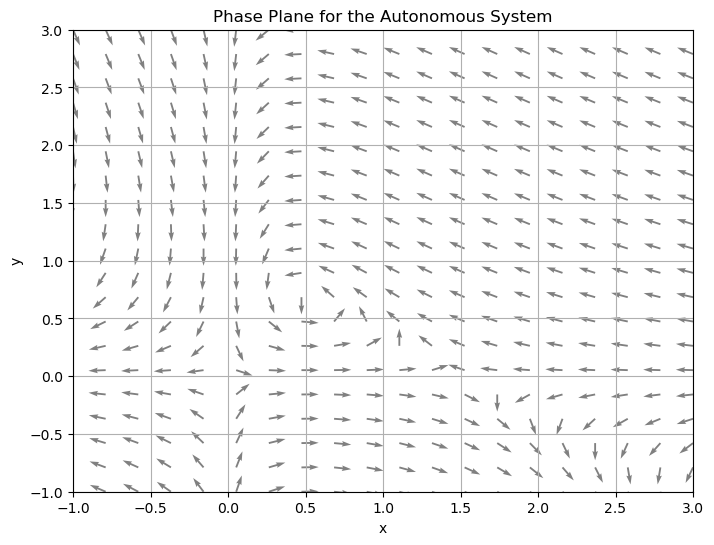
A phase plane for an autonomous system

\[ \frac{dx}{dt} = f(x,y) \]

\[ \frac{dy}{dt} = g(x,y) \]

is the grid \(\mathbb{R}^2\) in which vectors of the form

\[ \vec{v} = x'(t)\vec{i} + y'(t)\vec{j} = \langle f(x,y), g(x,y) \rangle \]

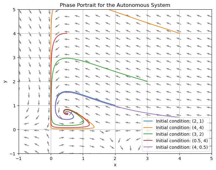
have been drawn at a set of grid points \((x_i,y_i)\). A phase portrait for the autonomous system is a phase plane with enough solution curves drawn in to show how solutions behave in every part of the plane.

Example

Draw a phase plane and then a phase portrait for the system

\[x' = x(3-2x)-3xy\]

\[y' = -y+2xy.\]

Show code cell source Hide code cell source

import numpy as np
import matplotlib.pyplot as plt

# Set the range of values for x and y
x = np.linspace(-1, 3, 20)
y = np.linspace(-1, 3, 20)

# Create a grid of points (x, y)
X, Y = np.meshgrid(x, y)

# Define the system of equations
dx = X*(3 - 2*X) - 3*X*Y
dy = -Y + 2*X*Y

# Normalize the arrows to have the same length
N = np.sqrt(dx**2 + dy**2)
dx = dx/N
dy = dy/N

# Create the quiver plot
plt.figure(figsize=(8, 6))
plt.quiver(X, Y, dx, dy, color='gray')

plt.title('Phase Plane for the Autonomous System')
plt.xlabel('x')
plt.ylabel('y')
plt.xlim([-1, 3])
plt.ylim([-1, 3])
plt.grid(True)
plt.show()

Show code cell source Hide code cell source

import numpy as np
import matplotlib.pyplot as plt
from scipy.integrate import odeint

# Define the range of values for x and y
x = np.linspace(-1, 5, 20)
y = np.linspace(-1, 5, 20)

# Create a grid of points (x, y)
X, Y = np.meshgrid(x, y)

# Define the system of equations
U = X*(3 - 2*X) - 3*X*Y
V = -Y + 2*X*Y

# Normalize the arrows to have the same length
N = np.sqrt(U**2 + V**2)
U = U/N
V = V/N

# Define the system for odeint
def dFdt(F, t):
    return [F[0]*(3 - 2*F[0]) - 3*F[0]*F[1], -F[1] + 2*F[0]*F[1]]

# Set the time points where the solution is computed
t = np.linspace(-10, 10, 1000)  # Negative times are included here

# Set a collection of initial conditions
initial_conditions = [(2, 1), (4, 4), (3, 2), (0.5, 4), (4, 0.5)]

# Create the quiver plot
plt.figure(figsize=(8, 6))
plt.quiver(X, Y, U, V, color='gray')

# Loop over each initial condition and plot the solution curve
for ic in initial_conditions:
    F = odeint(dFdt, ic, t)
    plt.plot(F[:, 0], F[:, 1], label=f'Initial condition: {ic}')

plt.title('Phase Portrait for the Autonomous System')
plt.xlabel('x')
plt.ylabel('y')
plt.xlim([-1, 5])
plt.ylim([-1, 5])
plt.grid(True)
plt.legend()
plt.show()

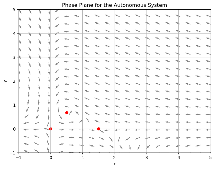
An equilibrium solution of an autonomous system

\[\frac{dx}{dt} = f(x,y)\]

\[\frac{dy}{dt} = g(x,y)\]

is a constant solution \(x(t) = \bar{x}\), \(y(t)=\bar{y}\) for which \(f(\bar{x}, \bar{y})\) and \(g(\bar{x},\bar{y})\) are simultaneously 0. The point in the phase plane corresponding to an equilibrium solution is called an equilibrium point.

Example

Find the equilibrium solutions of the system and plot those points in the phase plane

\[x' = x(3-2x)-3xy\]

\[y' = -y+2xy.\]

To find the equilibrium solutions, we need to solve the system

\[ 3x-2x^2-3xy=0 \rightarrow x(3-2x-3y)=0 \]

\[ -y+2xy=0 \rightarrow y(-1+2x)=0 \]

This tells us that either \(x=0\) OR \(3-2x-3y=0\) or \(y=0\) OR \(-1+2x=0\).

If \(x=0\), then \(y=0\). So \((0,0)\) is an equilibrium solution.

If \(y=0\) and \(x \neq 0\), then \(3-2x-3(0)=0 \rightarrow x=\frac{3}{2}\). So \(\left(\frac{3}{2},0\right)\) is an equilibrium solution.

If \(-1+2x=0 \rightarrow x=\frac{1}{2}\), then \(3-2\left(\frac{1}{2}\right)-3y=0 \rightarrow y=\frac{2}{3}\). So \(\left(\frac{1}{2},\frac{2}{3}\right)\) is the third and final equilibrium solution.

Show code cell source Hide code cell source

import numpy as np
import matplotlib.pyplot as plt
from scipy.integrate import odeint

# Define the range of values for x and y
x = np.linspace(-1, 5, 20)
y = np.linspace(-1, 5, 20)

# Create a grid of points (x, y)
X, Y = np.meshgrid(x, y)

# Define the system of equations
U = X*(3 - 2*X) - 3*X*Y
V = -Y + 2*X*Y

# Normalize the arrows to have the same length
N = np.sqrt(U**2 + V**2)
U = U/N
V = V/N

# Create the quiver plot
plt.figure(figsize=(8, 6))
plt.quiver(X, Y, U, V, color='gray')

# Plot the equilibrium points
equilibrium_points = [(0, 0), (3/2, 0), (1/2, 2/3)]
for eq_pt in equilibrium_points:
    plt.scatter(*eq_pt, color='red')

plt.title('Phase Plane for the Autonomous System')
plt.xlabel('x')
plt.ylabel('y')
plt.xlim([-1, 5])
plt.ylim([-1, 5])
plt.grid(True)
plt.show()

11.5.5. Geometric Behavior of Homogeneous Linear Systems

Let \(A\) be a \(2 \times 2\) matrix where \(A\) has two distinct real eigenvalues and consider the system \(x' = Ax\):

• \(x'=Ax\) has a unique solution for any initial condition \((x_0,y_0) \in \mathbb{R}^2\)

• If \(\det(A) \neq 0\), then \((0,0)\) is the only equilibrium solution of \(x' = Ax\)

• The lines spanned by the eigenvectors form straight line solution curves

• For large values of \(t\), solutions will tend twoards the straight line solution for the largest eigenvalue (sometimes called the dominant eigenvalue)

Subsequently, to describe the geometric behavior of the solutions, it is enough to draw the eigenvalue solutions, and one sample solution curve in each of the four regions.

Example

Consider the two-dimensional homogeneous linear system

\[\begin{split}x' = \begin{bmatrix} -4 & -2 \\ 1 & -1 \end{bmatrix}x\end{split}\]

which has eigenvalues \(\lambda_1 = -3\) and \(\lambda_2 = -2\) with respective eigenvectors

\[\begin{split} v_1 = \begin{bmatrix} -2 \\ 1 \end{bmatrix} \end{split}\]

and

\[\begin{split} v_2 = \begin{bmatrix} -1 \\ 1 \end{bmatrix}. \end{split}\]

Show code cell source Hide code cell source

import numpy as np
import matplotlib.pyplot as plt
from scipy.integrate import solve_ivp

# Define the system of equations
def system(t, state):
    x, y = state
    dx = -4*x -2*y
    dy = x - y
    return [dx, dy]

# Set up the grid
Y, X = np.mgrid[-10:10:20j, -10:10:20j]
DX, DY = system(None, [X, Y])

# Normalize vectors to a consistent length for visualization
M = (np.hypot(DX, DY))                           # Norm of the growth rate 
M[M == 0] = 1.                                 # Avoid zero division errors 
DX /= M                                        # Normalize each arrows
DY /= M

fig, ax = plt.subplots(figsize=(8, 8))

# Plot the vector field using quiver
ax.quiver(X, Y, DX, DY, M, pivot='mid')

# Define the eigenvalues and eigenvectors
lambda1 = -3
lambda2 = -2
v1 = np.array([-2, 1])
v2 = np.array([-1, 1])

x = np.linspace(-10, 10, 400)

# Plot the eigenvalue solutions
ax.plot(x, (v1[1]/v1[0]) * x, 'r', label='Eigenvalue λ1=-3')
ax.plot(x, (v2[1]/v2[0]) * x, 'b', label='Eigenvalue λ2=-2')

# Plot solution curves for two initial conditions
t_span = [-10, 10] # This will make the solution curves extend from t=-10 to t=10
t_eval = np.linspace(-10, 10, 400)
for initial_condition in [(3, 7), (-4, -4)]:
    sol = solve_ivp(system, t_span, initial_condition, t_eval=t_eval)
    ax.plot(sol.y[0], sol.y[1])

ax.set_xlabel('t')
ax.set_ylabel('x')
ax.grid(True)
ax.axvline(0, color='black',linewidth=0.5)
ax.axhline(0, color='black',linewidth=0.5)
plt.xlim([-10, 10])
plt.ylim([-10, 10])
ax.legend()
plt.show()

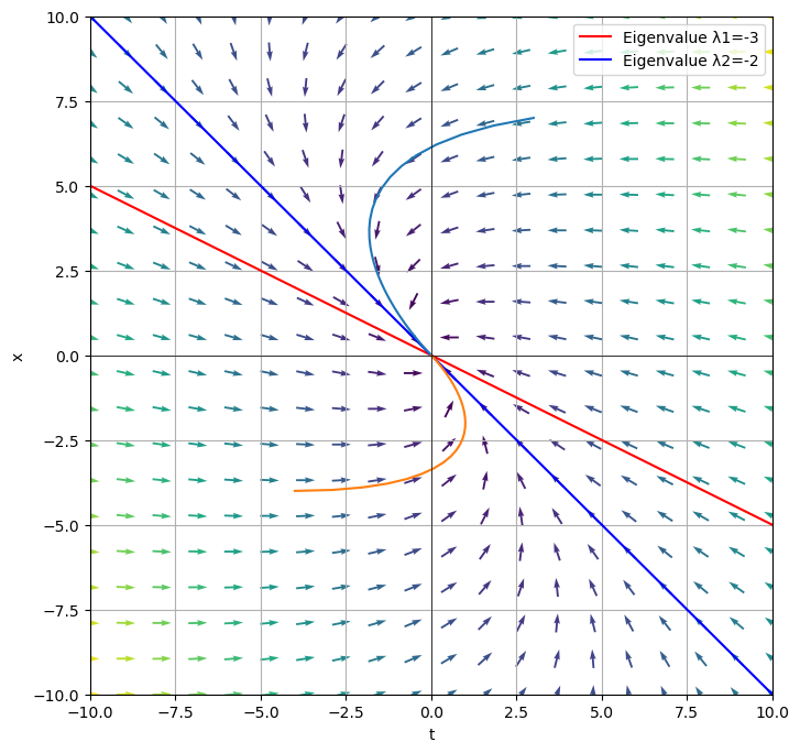
Notice that we can see from the phase plane that \((0,0)\) is a stable equilibrium. Also notice that as \(t \rightarrow \infty\), the solutions approach the stable equilibrium.

Example

Consider the two-dimensional homogeneous linear system

\[\begin{split}x' = \begin{bmatrix} 7 & 3 \\ 1 & 5 \end{bmatrix}x\end{split}\]

which has eigenvalues \(\lambda_1 = 4\) and \(\lambda_2 = 8\) with respective eigenvectors \(v_1 = \begin{bmatrix} -1 \\ 1 \end{bmatrix}\) and \(v_2 = \begin{bmatrix} 1 \\ \frac{1}{3} \end{bmatrix}\).

Show code cell source Hide code cell source

import numpy as np
import matplotlib.pyplot as plt
from scipy.integrate import solve_ivp

# Define the system of equations
def system(t, state):
    x, y = state
    dx = 7*x +3*y
    dy = x + 5*y
    return [dx, dy]

# Set up the grid
Y, X = np.mgrid[-10:10:20j, -10:10:20j]
DX, DY = system(None, [X, Y])

# Normalize vectors to a consistent length for visualization
M = (np.hypot(DX, DY))                           # Norm of the growth rate 
M[M == 0] = 1.                                 # Avoid zero division errors 
DX /= M                                        # Normalize each arrows
DY /= M

fig, ax = plt.subplots(figsize=(8, 8))

# Plot the vector field using quiver
ax.quiver(X, Y, DX, DY, M, pivot='mid')

# Define the eigenvalues and eigenvectors
lambda1 = 4
lambda2 = 8
v1 = np.array([-1, 1])
v2 = np.array([3, 1])

x = np.linspace(-10, 10, 400)

# Plot the eigenvalue solutions
ax.plot(x, (v1[1]/v1[0]) * x, 'r', label='Eigenvalue λ1=4')
ax.plot(x, (v2[1]/v2[0]) * x, 'b', label='Eigenvalue λ2=8')

# Plot solution curves for two initial conditions
t_span = [-10, 10] # This will make the solution curves extend from t=-10 to t=10
t_eval = np.linspace(-10, 10, 400)
for initial_condition in [(0.2, 0), (0, -0.2)]:
    sol = solve_ivp(system, t_span, initial_condition, t_eval=t_eval)
    ax.plot(sol.y[0], sol.y[1])

ax.set_xlabel('t')
ax.set_ylabel('x')
ax.grid(True)
ax.axvline(0, color='black',linewidth=0.5)
ax.axhline(0, color='black',linewidth=0.5)
plt.xlim([-10, 10])
plt.ylim([-10, 10])
ax.legend()
plt.show()

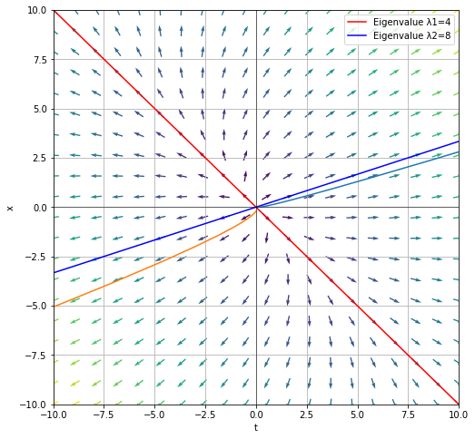
Notice that we can see from the phase plane that \((0,0)\) is an unstable equilibrium. Also notice that as \(t \rightarrow \infty\), the solutions approach \(\begin{bmatrix} 1 \\ \frac{1}{3} \end{bmatrix}e^{8t}\).

Example

Consider the two-dimensional homogeneous linear system

\[\begin{split}x' = \begin{bmatrix} 1 & 4 \\ 2 & -1 \end{bmatrix}x\end{split}\]

which has eigenvalues \(\lambda_1 = -3\) and \(\lambda_2 = 3\) with respective eigenvectors \(v_1 = \begin{bmatrix} -1 \\ 1 \end{bmatrix}\) and \(v_2 = \begin{bmatrix} 2 \\ 1 \end{bmatrix}\).

Show code cell source Hide code cell source

import numpy as np
import matplotlib.pyplot as plt
from scipy.integrate import solve_ivp

# Define the system of equations
def system(t, state):
    x, y = state
    dx = 1*x +4*y
    dy = 2*x - y
    return [dx, dy]

# Set up the grid
Y, X = np.mgrid[-10:10:20j, -10:10:20j]
DX, DY = system(None, [X, Y])

# Normalize vectors to a consistent length for visualization
M = (np.hypot(DX, DY))                           # Norm of the growth rate 
M[M == 0] = 1.                                 # Avoid zero division errors 
DX /= M                                        # Normalize each arrows
DY /= M

fig, ax = plt.subplots(figsize=(8, 8))

# Plot the vector field using quiver
ax.quiver(X, Y, DX, DY, M, pivot='mid')

# Define the eigenvalues and eigenvectors
lambda1 = -3
lambda2 = 3
v1 = np.array([-1, 1])
v2 = np.array([2, 1])

x = np.linspace(-10, 10, 400)

# Plot the eigenvalue solutions
ax.plot(x, (v1[1]/v1[0]) * x, 'r', label='Eigenvalue λ1=-3')
ax.plot(x, (v2[1]/v2[0]) * x, 'b', label='Eigenvalue λ2=3')

# Plot solution curves for two initial conditions
t_span = [-10, 10] # This will make the solution curves extend from t=-10 to t=10
t_eval = np.linspace(-10, 10, 400)
for initial_condition in [(-5, 7), (7, -6), (-9,8), (8,-9)]:
    sol = solve_ivp(system, t_span, initial_condition, t_eval=t_eval)
    ax.plot(sol.y[0], sol.y[1])

ax.set_xlabel('t')
ax.set_ylabel('x')
ax.grid(True)
ax.axvline(0, color='black',linewidth=0.5)
ax.axhline(0, color='black',linewidth=0.5)
plt.xlim([-10, 10])
plt.ylim([-10, 10])
ax.legend()
plt.show()

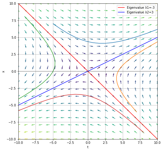
Notice that we can see from the phase plane that \((0,0)\) is a semi-stable equilibrium. In particular, if our initial condition started on \(\begin{bmatrix} -1 \\ 1 \end{bmatrix}e^{-3t}\), then it will tend towards zero. But if the initial condition does not lie on that line, then the solutions tends towards \(\begin{bmatrix} 2 \\ 1 \end{bmatrix}e^{3t}\).

Let \(A\) be a \(2 \times 2\) matrix where \(A\) has two complex eigenvalues, \(\lambda = a \pm bi\), and consider the system \(x' = Ax\):

• \(x'=Ax\) has a unique solution for any initial condition \((x_0,y_0) \in \mathbb{R}^2\)

• \((0,0)\) is the only equilibrium solution of \(x' = Ax\)

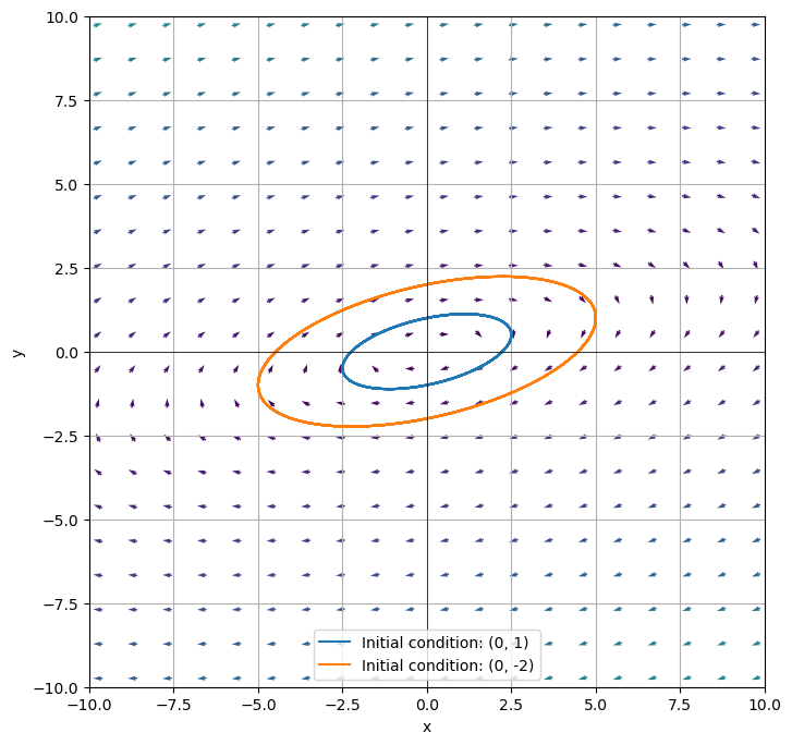
• If \(a=0\), the solutions are periodic and will form elliptic orbits around \((0,0)\)

• If \(a>0\), the solution curves will be elliptic spirals away from \((0,0)\)

• If \(a<0\), the solution curves will be elliptic spirals toward from \((0,0)\)

• The direction of the spiral (clockwise vs. counterclockwise) can be determined by checking a single test point.

In general, we care about the correct behavior and the correct spin. We do not need additional detail.

Example

Consider the two-dimensional homogeneous linear system

\[\begin{split}x' = \begin{bmatrix} -1 & 5 \\ -1 & 1 \end{bmatrix}x\end{split}\]

which has eigenvalues \(\lambda_1 = -2i\) and \(\lambda_2 = 2i\) with respective eigenvectors \(v_1 = \begin{bmatrix} 1-2i \\ 1 \end{bmatrix}\) and \(v_2 = \begin{bmatrix} 1+2i \\ 1 \end{bmatrix}\).

Show code cell source Hide code cell source

import numpy as np
import matplotlib.pyplot as plt
from scipy.integrate import solve_ivp

# Define the system of equations
def system(t, state):
    x, y = state
    dx = -1*x + 5*y
    dy = -1*x + y
    return [dx, dy]

# Set up the grid
Y, X = np.mgrid[-20:20:40j, -20:20:40j]
DX, DY = system(None, [X, Y])

# Normalize vectors to a consistent length for visualization
M = (np.hypot(DX, DY))
M[M == 0] = 1.
DX /= M
DY /= M

fig, ax = plt.subplots(figsize=(8, 8))

# Plot the vector field using quiver
ax.quiver(X, Y, DX, DY, M, pivot='mid')

# Define the eigenvalues and eigenvectors
lambda1 = -2j
lambda2 = 2j
v1 = np.array([1-2j, 1])
v2 = np.array([1+2j, 1])

x = np.linspace(-10, 10, 800)

# Plot solution curves for two initial conditions
t_span = [-10, 10]
t_eval = np.linspace(t_span[0], t_span[1], 1000)

for initial_condition in [(0, 1), (0, -2)]:
    sol = solve_ivp(system, t_span, initial_condition, t_eval=t_eval)
    ax.plot(sol.y[0], sol.y[1],label=f'Initial condition: {initial_condition}')

ax.set_xlabel('x')
ax.set_ylabel('y')
ax.grid(True)
ax.axvline(0, color='black',linewidth=0.5)
ax.axhline(0, color='black',linewidth=0.5)
plt.xlim([-10, 10])
plt.ylim([-10, 10])
ax.legend()
plt.show()

Example

Consider the two-dimensional homogeneous linear system

\[\begin{split}x' = \begin{bmatrix} -2 & 5 \\ -1 & 0 \end{bmatrix}x\end{split}\]

which has eigenvalues \(\lambda_1 = -1-2i\) and \(\lambda_2 = -1+2i\) with respective eigenvectors \(v_1 = \begin{bmatrix} 1+2i \\ 1 \end{bmatrix}\) and \(v_2 = \begin{bmatrix} 1-2i \\ 1 \end{bmatrix}\).

Show code cell source Hide code cell source

import numpy as np
import matplotlib.pyplot as plt
from scipy.integrate import solve_ivp

# Define the system of equations
def system(t, state):
    x, y = state
    dx = -2*x + 5*y
    dy = -1*x
    return [dx, dy]

# Set up the grid
Y, X = np.mgrid[-20:20:40j, -20:20:40j]
DX, DY = system(None, [X, Y])

# Normalize vectors to a consistent length for visualization
M = (np.hypot(DX, DY))
M[M == 0] = 1.
DX /= M
DY /= M

fig, ax = plt.subplots(figsize=(8, 8))

# Plot the vector field using quiver
ax.quiver(X, Y, DX, DY, M, pivot='mid')

# Define the eigenvalues and eigenvectors
lambda1 = -1-2j
lambda2 = -1+2j
v1 = np.array([1+2j, 1])
v2 = np.array([1-2j, 1])

x = np.linspace(-10, 10, 800)

# Plot solution curves for two initial conditions
t_span = [-10, 10]
t_eval = np.linspace(t_span[0], t_span[1], 1000)

for initial_condition in [(7, 7), (-3, -6)]:
    sol = solve_ivp(system, t_span, initial_condition, t_eval=t_eval)
    ax.plot(sol.y[0], sol.y[1],label=f'Initial condition: {initial_condition}')

ax.set_xlabel('x')
ax.set_ylabel('y')
ax.grid(True)
ax.axvline(0, color='black',linewidth=0.5)
ax.axhline(0, color='black',linewidth=0.5)
plt.xlim([-10, 10])
plt.ylim([-10, 10])
ax.legend()
plt.show()

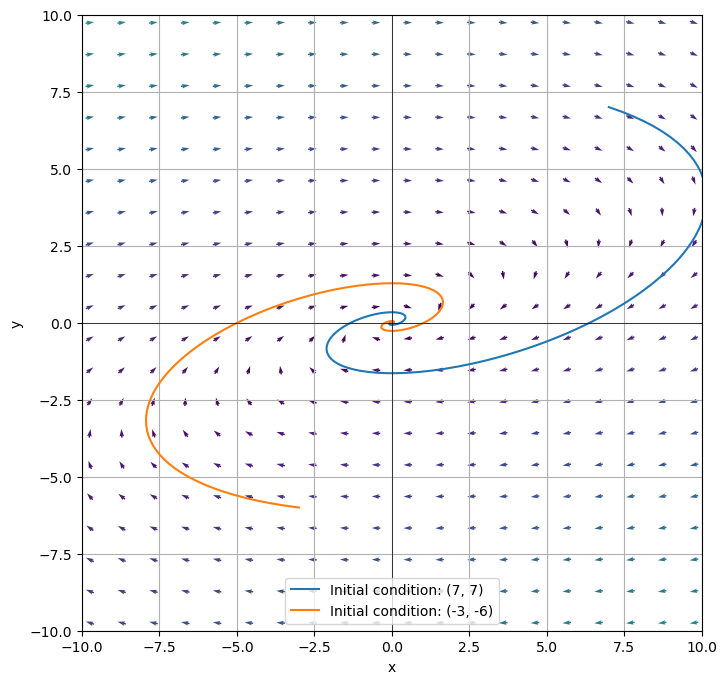
Notice in this case, \(\text{Re}(\lambda) = -1 <0\), which tells us the spiral will move towards \((0,0)\). We call this a spiral stable equilibrium. If \(\text{Re}(\lambda) > 0\), the spiral will move away from \((0,0)\) and is called a spiral unstable equilibrium (See Exercise 10).

11.5.6. The Phase Plane for Nonlinear Autonomous Systems

The goal of this section is to understand the behavior of nonlinear systems of differential equations by sketching the phase plane.

Given an autonomous system

\[x' = f(x,y)\]

\[y' = g(x,y)\]

the nullclines for \(x'\) are the set of all the curves where \(x'=0\), which can be found by solving \(f(x,y)=0\) explicitly (if possible). Similarly, the nullclines for \(y'\) are the set of all curves where \(y'=0\). Note that on \(x'\) nullclines, tangent vectors are vertical and on \(y'\) nullclines, tangent vectors are horizontal.

In addition, these nullclines encode the equilibrium solutions. These occur at the intersection of the \(x'\) and \(y'\) nullclines. Moreover, the arrows on the nullclines can only switch direction at an equilibrium point, that is, the intersection points, listed above.

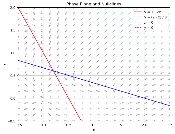
Example

Find the nullclines for the system

\[x' = x(2-x)-3xy\]

\[y' = y(1-y)-2xy.\]

To find the nullclines, we set each equation equal to zero.

When \(x'=0\): \(x(2-x-3y)=0 \rightarrow x=0 \text{ or } y= \dfrac{2-x}{3}\). These are the \(x'\) nullclines.

When \(y'=0\): \(y(1-y-2x)=0 \rightarrow y=0 \text{ or } y= 1-2x\). These are the \(y'\) nullclines.

Notice that from these nullclines, we can also find the equilibrium solutions, by figuring out the intersection points. Notice that \((0,0)\) is an equilibrium solution corresponding to \(x=0\), \(y=0\). \((0,1)\) is an eqilibrium solution corresponding to \(x=0\), \(y=1-2x\). \((2,0)\) is an equilibrium solution corresponding to \(y=\dfrac{2-x}{3}\), \(y=0\). The last equilibrium solution is \(\left(\dfrac{1}{5}, \dfrac{3}{5} \right)\), which corresponds to \(y= \dfrac{2-x}{3}\), \(y=1-2x\).

Show code cell source Hide code cell source

import numpy as np
import matplotlib.pyplot as plt

# Define the system of equations
def system(x, y):
    dx = x * (2 - x) - 3 * x * y
    dy = y * (1 - y) - 2 * x * y
    return dx, dy

# Create an x, y grid
y, x = np.mgrid[-0.5:2:20j, -0.5:2.5:20j]

# Calculate dx, dy for the vector field
dx, dy = system(x, y)

# Normalize the arrows so their size represents their speed
M = (np.hypot(dx, dy))                           
M[M == 0] = 1.                                 
dx /= M                                        
dy /= M

plt.figure(figsize=(8, 6))

# Plot the vector field using quiver
plt.quiver(x, y, dx, dy, M, pivot='mid', alpha=0.5)

# Create an x vector
x = np.linspace(-0.5, 2.5, 200)

# Define nullclines
y1 = 1 - 2 * x
y2 = (2 - x) / 3

# Plot nullclines
plt.plot(x, y1, 'r', label="y = 1 - 2x")
plt.plot(x, y2, 'b', label="y = (2 - x) / 3")

# Also plot x=0 and y=0
plt.axvline(0, color='green', linestyle='--', label="x = 0")
plt.axhline(0, color='purple', linestyle='--', label="y = 0")

# Labels and legends
plt.xlabel('x')
plt.ylabel('y')
plt.legend()

# Set the x and y axis cutoffs
plt.ylim([-0.5,2])
plt.xlim([-0.5,2.5])

plt.grid(True)
plt.title('Phase Plane and Nullclines')
plt.show()

Given an autonomous system

\[x' = f(x,y)\]

\[y' = g(x,y)\]

with equilibrium point \((a,b)\), the linearization of the system at \((a,b)\) is the linear system

\[\begin{split} \begin{bmatrix} x' \\ y' \end{bmatrix} = \begin{bmatrix} \dfrac{\partial f}{\partial x} \bigm|_{(a,b)} & \dfrac{\partial f}{\partial y} \bigm|_{(a,b)} \\ \dfrac{\partial g}{\partial x} \bigm|_{(a,b)} & \dfrac{\partial g}{\partial y} \bigm|_{(a,b)} \end{bmatrix} \begin{bmatrix} x-a \\ y-b \end{bmatrix}.\end{split}\]

In addition,

\[\begin{split}\begin{bmatrix} \dfrac{\partial f}{\partial x} & \dfrac{\partial f}{\partial y} \\ \dfrac{\partial g}{\partial x} & \dfrac{\partial g}{\partial y} \end{bmatrix} \end{split}\]

is called the Jacobian Matrix of the system and is typically denoted \(J(x,y)\). If we want to evaluate it at a point, (a,b), as is done in the linearization defintion, we denote that \(J(a,b)\).

Example (cont.)

Find the linearization of the system

\[x' = x(2-x)-3xy\]

\[y' = y(1-y)-2xy\]

at each of its equilibrium solutions.

Recall from the work done previously that the equilibrium solutions are \((0,0)\), \((0,1)\), \((2,0)\), and \(\left(\dfrac{1}{5}, \dfrac{3}{5} \right)\).

Now we want to find the Jacobian Matrix, \(J(x,y)\).

\[\begin{split}J(x,y) = \begin{bmatrix} \dfrac{\partial }{\partial x}(2x-x^2-3xy) & \dfrac{\partial }{\partial y}(2x-x^2-3xy) \\ \dfrac{\partial }{\partial x}(y-y^2-2xy) & \dfrac{\partial }{\partial y}(y-y^2-2xy) \end{bmatrix} = \begin{bmatrix} 2-2x-3y & -3x \\ -2y & 1-2y-2x \end{bmatrix}\end{split}\]

So the linearization of \((0,0)\) is

\[\begin{split} \begin{bmatrix} x' \\ y' \end{bmatrix} = J(0,0) \begin{bmatrix} x-0 \\ y-0 \end{bmatrix} = \begin{bmatrix} 2 & 0 \\ 0 & 1 \end{bmatrix}\begin{bmatrix} x \\ y \end{bmatrix}\end{split}\]

So the linearization of \((0,1)\) is

\[\begin{split} \begin{bmatrix} x' \\ y' \end{bmatrix} = J(0,1) \begin{bmatrix} x-0 \\ y-1 \end{bmatrix} = \begin{bmatrix} -1 & 0 \\ -2 & -1 \end{bmatrix}\begin{bmatrix} x \\ y-1 \end{bmatrix}\end{split}\]

So the linearization of \((2,0)\) is

\[\begin{split} \begin{bmatrix} x' \\ y' \end{bmatrix} = J(2,0) \begin{bmatrix} x-2 \\ y-0 \end{bmatrix} = \begin{bmatrix} -2 & -6 \\ 0 & -3 \end{bmatrix}\begin{bmatrix} x-2 \\ y \end{bmatrix}\end{split}\]

So the linearization of \(\left(\dfrac{1}{5}, \dfrac{3}{5} \right)\) is

\[\begin{split} \begin{bmatrix} x' \\ y' \end{bmatrix} = J\left(\dfrac{1}{5}, \dfrac{3}{5} \right) \begin{bmatrix} x-\dfrac{1}{5} \\ y - \dfrac{3}{5} \end{bmatrix} = \begin{bmatrix} -\dfrac{1}{5} & -\dfrac{3}{5} \\ -\dfrac{6}{5} & -\dfrac{3}{5} \end{bmatrix}\begin{bmatrix} x-\dfrac{1}{5} \\ y - \dfrac{3}{5} \end{bmatrix}\end{split}\]

Consider the linearization of \((2,0)\) found above

\[\begin{split} \begin{bmatrix} x' \\ y' \end{bmatrix} = \begin{bmatrix} -2 & -6 \\ 0 & -3 \end{bmatrix}\begin{bmatrix} x-2 \\ y \end{bmatrix}. \end{split}\]

Our hope is that the behavior of a nonlinear system is similar locally to the behavior of the linear system. In this case the eigenvalues of

\[\begin{split} \begin{bmatrix} -2 & -6 \\ 0 & -3 \end{bmatrix} \end{split}\]

are \(\lambda = -2\) and \(\lambda=-3\). So we hope that locally our system behaves like a sink near \((2,0)\). Looking back at the nullclines phase plane, we do see that it behaves like a sink near \((2,0)\). It turns out that most of the time linearization describes local behavior at an equilibrium, but not always. The next result by Hartman and Grobman discusses when we can expect the linearization to describe local behavior.

Theorem (Hartman-Grobman Theorem)

Given a nonlinear autonomous system

\[x' = f(x,y)\]

\[y' = g(x,y)\]

with equilibrium point \((a,b)\), suppose that for any eigenvalue \(\lambda\) of \(J(a,b)\) we have \(\text{Re}(\lambda) \neq 0.\) Then the linearization

\[\begin{split}\begin{bmatrix} x' \\ y' \end{bmatrix} = J(a,b) \begin{bmatrix} x-a \\ y-b \end{bmatrix}\end{split}\]

describes the qualitative behavior of the system near the equilibrium point \((a,b)\). This means that if \(\text{Re}(\lambda) = 0\), then linearization cannot be used to describe the local behavior.

11.5.7. Exercises

Exercises

1. Which of the following sets are linearly independent?

• \(\biggl\{\begin{bmatrix} e^{2t} \\ e^{4t} \end{bmatrix}, \begin{bmatrix} e^{2t} \\ e^{7t} \end{bmatrix}\biggr\}\)

• \(\biggl\{\begin{bmatrix} \cos(t) \\ -e^{3t} \end{bmatrix}, \begin{bmatrix} -\cos(t) \\ e^{3t} \end{bmatrix}\biggr\}\)

• \(\biggl\{v_1(t) = \begin{bmatrix} \sin^2(4t) \\ t \end{bmatrix}, v_2(t)= \begin{bmatrix} \cos^2(4t) \\ 3t \end{bmatrix}, v_3(t) = \begin{bmatrix} 1 \\ 4t \end{bmatrix}\biggr\}\)

2. Solve the initial-value problem \( x' = \begin{bmatrix} -3 & 1 & -1 \\ 0 & -3 & 2 \\ 0 & -1 & 0 \end{bmatrix}x, \quad x(0) = \begin{bmatrix} 1 \\ 1 \\ 0 \end{bmatrix}. \)

3. Solve the initial-value problem \( x' = \begin{bmatrix} 4 & -1 & 3 \\ 0 & 4 & -2 \\ 0 & 0 & 2 \end{bmatrix}x, \quad x(0) = \begin{bmatrix} 0 \\ 0 \\ 2 \end{bmatrix}. \)

4. Find the general solution to the linear system of differential equations \( x' = \begin{bmatrix} -1 & 0 & 10 \\ 0 & 2 & 1 \\ 0 & -1 & 2 \end{bmatrix}x. \)

5. Solve the initial-value problem \( x' = \begin{bmatrix} 2 & 0 & -3 \\ 1 & 1 & -1 \\ 0 & 0 & -1 \end{bmatrix}x + \begin{bmatrix}3e^{-2t} \\ 6e^{-2t} \\ 3e^{-2t} \end{bmatrix}, \quad x(0) = \begin{bmatrix} 1 \\ 0 \\ 2 \end{bmatrix}. \)

6. Which of the following systems are autonomous?

• \(\begin{cases}x' = x^2y+y-x \\ y' = xt+yt-xy\end{cases}\).

• \(\begin{cases}x' = y-x \\ y' = x+y\end{cases}\).

7. When are homogeneous linear systems with constant coefficients autonomous? That is, when is \(x'=Ax\) autonomous?

8. When are nonhomogeneous linear systems with constant coefficients autonomous? That is, when is \(x'=Ax+b\) autonomous?

9. Plot a phase plane for the system \(x' = x(7-2x)-4xy\), \( \) \(y' = -y+2xy.\)

10. Consider the two-dimensional homogeneous linear system \(x' = \begin{bmatrix} 0 & 10 \\ -1 & 2 \end{bmatrix}x.\) Find eigenvalues and their respective eigenvectors and use this information to plot a phase plane with two sample solution curves.

11. Consider the nonlinear autonomous system \(x' = x(5-x)-4xy\), \( \) \(y' = y(3-y)-2xy.\) Find the nullclines and equilibrium points and plot a phase plane. Then find the linearization at each equilibrium solution, and if possible, use that linearization to describe the qualitative behavior near each equilibrium solution.