8.3. Limits, Continuity, and Rates#
Note
Below is the list of topics that are covered in this section:
Limits
Continuity
Measures of Change over an Interval
Measures of Change at a Point
Secant and Tangent Lines
import sympy as sp
from scipy.optimize import fsolve
import numpy as np
import matplotlib.pyplot as plt
import math
8.3.1. Limits#
In the previous section, while talking about behaviors of some common functions, we saw the phrase “\(f(x)\) goes to \(\infty\) as \(x\) goes to \(\infty\)”.
This phrase describes how the output of a function behaves as the input is approaching something and can be written using limit notation: \(\lim\limits_{x\to\infty}f(x)=\infty\).
The keyword here is “approaching”. The input is not equal to a certain point, it is approaching it.
We say that the limit of \(f(x)\) is \(L\) as \(x\) approaches \(a\) and write this as \(\lim\limits_{x\to a}f(x)=L\) provided we can make \(f(x)\) as close to \(L\) as needed for all \(x\) sufficiently close to \(a\), from both sides, without actually letting \(x\) be \(a\).
\(\lim\limits_{x\to a}f(x)=L\) can also alternatively be written as \(f(x) \to L \text{ as } x\to a\).
The phrase “from both sides” refer to the Left-hand limits and Right-hand limits.
For function \(f\) defined on an interval containing a constant \(a\) (except possibly at \(a\) itself):
Left-hand limit of \(f\) as \(x\) approaches \(a\) from the left is written \(\lim\limits_{x\to a^-}f(x)=L_1\)
Right-hand limit of \(f\) as \(x\) approaches \(a\) from the right is written \(\lim\limits_{x\to a^+}f(x)=L_2\)
Here \(a^-\) denotes “to the left of \(a\) and \(a^+\) denotes “to the right of \(a\).
By definition, for function \(f\) defined on an interval containing a constant \(a\) (except possibly at \(a\) itself), the limit of \(f\) as \(x\) approaches \(a\) exists if and only if \(\lim\limits_{x\to a^-}f(x)=\lim\limits_{x\to a^+}f(x)=L\), and hence written \(\lim\limits_{x\to a}f(x)=L\)
Example 1
Given the graph of \(f(x)\) below:
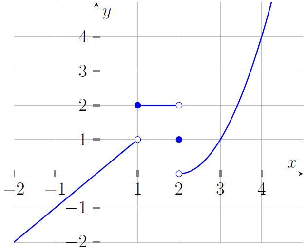
\(\lim\limits_{x\to 0^-}f(x)=0\) while \(\lim\limits_{x\to 0^+}f(x)=0\) hence \(\lim\limits_{x\to 0}f(x)=0\).
\(\lim\limits_{x\to 1^-}f(x)=1\) while \(\lim\limits_{x\to 1^+}f(x)=2\) hence \(\lim\limits_{x\to 1}f(x)\) does not exists.
Note that when looking for limits as \(x\) approaching \(0\) or \(1\), it never mattered what \(f(0)\) or \(f(1)\) is, as we only see the values to the left and right of those points.
Below is a code example that prompt user for a function \(f(x)\) and a constant \(a\), and then return \(\lim\limits_{x\to a}f(x)=L\).
Show code cell source
# Prompt the user to input the function f(x) and the constant a
expression_str = input("Enter the function f(x): ")
a = float(input("Enter the constant a: "))

# Define the variable x and the function f(x)
x = sp.symbols('x')
f_x = sp.sympify(expression_str)

# Calculate the limit of f(x) as x approaches a
limit_result = sp.limit(f_x, x, a)

# Print the result
print("The limit of f(x) as x approaches", a, "is:", limit_result)
The limit of f(x) as x approaches 3.8 is: -2.44743156377088
Limit Properties#
Assuming \(\lim\limits_{x\to a}f(x)\) and \(\lim\limits_{x\to a}g(x)\) exists and \(c\) is any constant. Then:
\(\lim\limits_{x\to a}\left[c\cdot f(x)\right]=c\cdot \lim\limits_{x\to a}f(x)\)
\(\lim\limits_{x\to a}\left[f(x) \pm g(x)\right]=\lim\limits_{x\to a}f(x) \pm \lim\limits_{x\to a}g(x)\)
\(\lim\limits_{x\to a}\left[f(x) \cdot g(x)\right]=\lim\limits_{x\to a}f(x) \cdot \lim\limits_{x\to a}g(x)\)
\(\lim\limits_{x\to a}\left[\dfrac{f(x)}{g(x)}\right]= \frac{\lim\limits_{x\to a}f(x)}{\lim\limits_{x\to a}g(x)}\), provided \(\lim\limits_{x\to a}g(x)\neq 0\)
\(\lim\limits_{x\to a}\left[f(x)\right]^n=\left[\lim\limits_{x\to a}f(x)\right]^n\)
\(\lim\limits_{x\to a} c=c\)
\(\lim\limits_{x\to a} x=a\)
8.3.2. Continuity#
Graphically, a function is continuous if it can be drawn without lifting the writing utensil from the paper.
Mathematically, a function \(f\) is continuous at \(\boldsymbol{x=a}\) if and only if the following three conditions are satisfied:
\(f(a)\) exists
\(\lim\limits_{x\to a}f(x)\) exists
\(\lim\limits_{x\to a}f(x)=f(a)\)
A function is continuous on an interval if these three conditions are met for every input value in the interval.
Fact: If \(\lim\limits_{x\to a}g(x)=b\) and \(f(x)\) is continuous at \(x=b\), then \(\lim\limits_{x\to a}f(g(x))=f\left(\lim\limits_{x\to a}g(x)\right)\).
Example
Evaluate \(\lim\limits_{x\to 0}e^{\cos(x)}\).
The function \(\cos(x)\) is continuous at \(x=0\) since \(\cos(0)=\lim\limits_{x\to 0^-}\cos(x)=\lim\limits_{x\to 0^+}\cos(x)=1\).
Hence \(\lim\limits_{x\to 0}e^{\cos(x)}=e^{\left(\lim\limits_{x\to 0}\cos(x)\right)}=e^1=e\). Of course, this can easily be checked using the code.
Show code cell source
# Define the variable x
x = sp.symbols('x')

# Define the function e^(cos(x))
f_x = sp.exp(sp.cos(x))

# Calculate the limit of e^(cos(x)) as x approaches 0
limit_result = sp.limit(f_x, x, 0)

# Print the result
print("The limit of e^(cos(x)) as x approaches 0 is:", limit_result)
The limit of e^(cos(x)) as x approaches 0 is: E
Intermediate Value Theorem#
Suppose that \(f(x)\) is continuous on \([a,b]\) and let \(M\) be any number between \(f(a)\) and \(f(b)\). Then there exists a constant \(c\) such that \(a<c<b\) and \(f(c)=M\).
Example
Show that the function \(f(x)=x^3+2x^2-0.3\) has a zero in the interval \([0,1]\).
Since \(f(x)\) is a polynomial, it is continuous everywhere. \(f(0)=-0.3\) and \(f(1)=2.7\).
Since \(0\) is between \(-0.3\) and \(2.7\), then by the Intermediate Value Theorem, there is a constant \(c\) between \(0\) and \(1\) such that \(f(c)=0\), that is, \(c\) is a zero of \(f(x)\) on \([0,1]\).
This theorem can be useful for computationally expensive functions. Otherwise, with the help of any calculating tools, it is quite simple to just find all the zeros of a given function in a given interval. Below is a code example that prompts the user for \(f(x)\) and interval \([a,b]\), and then returns the zeroes located in \([a,b]\).
Show code cell source
# Prompt the user to input the function f(x)
expression_str = input("Enter the function f(x): ")
f_x = lambda x: eval(expression_str)

# Prompt the user to input the interval [a, b]
a = float(input("Enter the lower bound of the interval (a): "))
b = float(input("Enter the upper bound of the interval (b): "))

# Define a function to check if a value is within the interval [a, b]
def within_interval(x):
    return a <= x <= b

# Find all the zeros of the function within the interval [a, b]
zeros = set()
tolerance = 1e-6  # Adjust the tolerance as needed
for x0 in range(int(a), int(b)+1):
    zero = fsolve(f_x, x0)
    if within_interval(zero) and abs(zero) > tolerance:
        zeros.add(round(zero[0], 3))  # Round to three decimal places

# Print the zeros within the interval
print("Zeros of the function within the interval [a, b]:", zeros)
Zeros of the function within the interval [a, b]: {-0.438, 0.357, -1.918}
8.3.3. Measures of Change over an Interval#
If \(x_1\) and \(x_2\) are input values for the function \(f\) and \(x_1<x_2\), then:
the change in \(f\) from \(x_1\) to \(x_2\) is \(f(x_2)-f(x_1)\)
what it calculates: between input \(x_1\) and \(x_2\), by how much does the output changes?
the percent change in \(f\) from \(x_1\) to \(x_2\) is \(\dfrac{f(x_2)-f(x_1)}{f(x_1)}\cdot 100\%\)
what it calculates: between input \(x_1\) and \(x_2\), by how many % does the output changes?
the average rate of change (aRoC) in \(f\) from \(x_1\) to \(x_2\) is \(\dfrac{f(x_2)-f(x_1)}{x_2-x_1}\)
what it calculates: between input \(x_1\) and \(x_2\), how fast does the output changes?
Below is an example of code that prompt user to input two points \((x_1,f(x_1))\) and \((x_2,f(x_2))\), then return the change, percent change, and average rate of change between the two points.
Show code cell source
# Prompt the user to input the coordinates of the first point (x1, f(x1))
x1 = float(input("Enter the x-coordinate of the first point: "))
f_x1 = float(input("Enter the y-coordinate of the first point: "))

# Prompt the user to input the coordinates of the second point (x2, f(x2))
x2 = float(input("Enter the x-coordinate of the second point: "))
f_x2 = float(input("Enter the y-coordinate of the second point: "))

# Calculate the change, percent change and average rate of change
change = f_x2 - f_x1
percent_change = (change / f_x1) * 100
average_rate_of_change = change / (x2 - x1)

# Print the results
print("Change in y:", change)
print("Percent change:", percent_change, "%")
print("Average rate of change:", average_rate_of_change)
Change in y: 30.0
Percent change: 150.0 %
Average rate of change: 15.0
8.3.4. Measures of Change at a Point#
If \(x\) is an input values for the function \(f\), then:
the (instantaneous) rate of change (RoC) of \(f\) at point \(x=a\) is \(\lim\limits_{x\to a} \dfrac{f(x)-f(a)}{x-a}\)
what it calculates: at the input \(x=a\), how fast does the output changes?
the percent rate of change of \(f\) at point \(x=a\) is \(\dfrac{\text{RoC}}{f(a)}\cdot 100\%\)
what it calculates: at the input \(x=a\), how fast does the output percentage changes?
Below is an example of code that prompts the user to input a function \(f(x)\) and the point \(x=a\), then return the instantaneous rate of change and percent rate of change of \(f\) at \(x=a\).
Show code cell source
#this code is not using derivatives as we are still in Section 3.
# Prompt the user to input the function f(x)
expression_str = input("Enter the function f(x): ")
f_x = lambda x: eval(expression_str)

# Prompt the user to input the point a
a = float(input("Enter the value of a: "))

# Calculate the approximate instantaneous rate of change
delta_x = 0.0001  # Small interval
f_a = f_x(a)
f_a_plus_delta_x = f_x(a + delta_x)
instantaneous_rate_of_change = round((f_a_plus_delta_x - f_a) / delta_x, 3)

# Calculate the approximate percent rate of change
percent_rate_of_change = round((instantaneous_rate_of_change / f_a) * 100, 3)

# Print the results
print("Approximate Instantaneous Rate of Change:", instantaneous_rate_of_change)
print("Approximate Percent Rate of Change:", percent_rate_of_change)
Approximate Instantaneous Rate of Change: 28.0
Approximate Percent Rate of Change: 38.889
8.3.5. Secant and Tangent Lines#
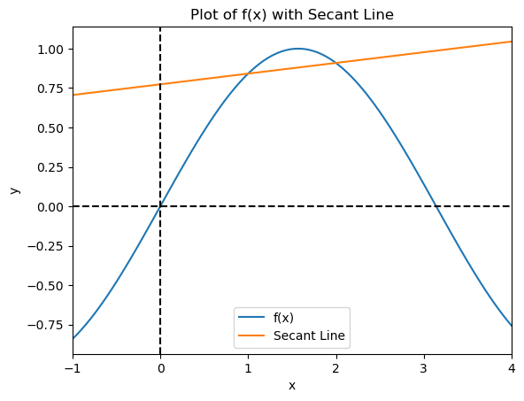
Given a continuous function \(f(x)\) on the interval containing \(x=a\) and \(x=b\), the secant line on \(f\) between \(x=a\) and \(x=b\) is a straight line connecting \((a,f(a))\) and \((b,f(b))\).
The slope of the secant line is the average rate of change of \(f\) between \(x=a\) and \(x=b\).
Below is an example code prompting the user to input function \(f\) as well as \(x=a\) and \(x=b\). Code will return the plot of \(f\) together with its secant line between \(x=a\) and \(x=b\).
Show code cell source
# Prompt user for a function f(x)
equation = input("Enter the function f(x): ")

# Define the function f(x)
def f(x):
    return eval(equation)

# Define the secant line function
def secant_line(x, a, b):
    return f(a) + (f(b) - f(a))/(b - a) * (x - a)

# Prompt user for values
a = float(input("Enter the value of a: "))
b = float(input("Enter the value of b: "))

# Generate x values
x = np.linspace(a - 2, b + 2, 100)

# Generate y values for f(x)
y = [f(val) for val in x]

# Generate y values for the secant line
secant = secant_line(x, a, b)

# Plot the function f(x) and the secant line
plt.plot(x, y, label='f(x)')
plt.plot(x, secant, label='Secant Line')

# Add the x=0 and y=0 axes
plt.axhline(0, color='black', linestyle='--')
plt.axvline(0, color='black', linestyle='--')

# Set the x-axis and y-axis labels
plt.xlabel('x')
plt.ylabel('y')

# Set the title
plt.title('Plot of f(x) with Secant Line')

# Set the legend
plt.legend()

# Set the x-axis limits
plt.xlim(a - 2, b + 2)

# Display the plot
plt.show()
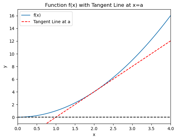
The word tangent comes from the Latin word tangere, meaning “to touch”.
Given a continuous function \(f(x)\) on the interval containing \(x=a\), the tangent line on \(f\) at \(x=a\) is a straight line touching \(f(x)\) at exactly \((a,f(a))\) and nowhere else.
The slope of this tangent line is the instantaneous rate of change of \(f\) at \(x=a\).
Below is an example code prompting user to input function \(f\) and \(x=a\). Code will return the plot of \(f\) together with its tangent line at \(x=a\).
Show code cell source
# Prompt the user to input the function f(x)
equation = input("Enter the function f(x): ")

# Prompt the user to input the value of a
a = float(input("Enter the value of a: "))

# Define the function f(x)
def f(x):
    return eval(equation)

# Generate x values for plotting
x = np.linspace(a - 2, a + 2, 100)

# Generate y values for the function f(x)
y = f(x)

# Calculate the tangent line at x = a
tangent_x = np.linspace(a - 2, a + 2, 100)
tangent_y = f(a) + (tangent_x - a) * (f(a + 0.01) - f(a)) / (0.01)

# Initialize the figure and axes
fig, ax = plt.subplots()

# Plot the function f(x)
ax.plot(x, y, label='f(x)')

# Plot the tangent line at x = a
ax.plot(tangent_x, tangent_y, 'r--', label='Tangent Line at a')

# Add the x=0 and y=0 axes
ax.axhline(0, color='black', linestyle='--')
ax.axvline(0, color='black', linestyle='--')

# Set the x-axis and y-axis limits
ax.set_xlim(a - 2, a + 2)
ax.set_ylim(min(y) - 1, max(y) + 1)

# Set the x-axis and y-axis labels
ax.set_xlabel('x')
ax.set_ylabel('y')

# Set the title
ax.set_title('Function f(x) with Tangent Line at x=a')

# Set the legend
ax.legend()

# Display the plot
plt.show()
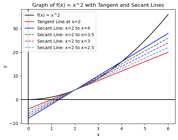
The tangent line at \(x=a\) can be obtained by taking the secant line between \(x=a\) and \(x=b\), then bring \(b\) closer and closer to \(a\).
Taking \(b=a+h\), the slope of the secant line between \(x=a\) and \(x=b\) is \(\dfrac{f(a+h)-f(a)}{a+h-a}=\dfrac{f(a+h)-f(a)}{h}\).
Bringing \(b \to a\) is then bringing \(h\to 0\), and hence the slope of the tangent line at \(x=a\) is \(\lim\limits_{h \to 0}\dfrac{f(a+h)-f(a)}{h}\). This realization is important as we introduce derivatives in the next section.
Below is the code showing the graph of \(f(x)=x^2\) with the secant lines between \(x=2\) and \(x=b\), starting from \(b=4\) until \(b=2\), which gives the tangent line of \(f(x)\) at \(x=2\).
Show code cell source
# Define the function f(x)
def f(x):
    return x**2

# Define the tangent line function at x = 2
def tangent_line(x):
    return 4 * (x - 2) + 4

# Define the secant line function
def secant_line(x, a, b):
    return (f(b) - f(a)) / (b - a) * (x - a) + f(a)

# Generate x values for plotting
x = np.linspace(0, 6, 100)

# Generate y values for the function f(x)
y = f(x)

# Generate y values for the tangent line at x = 2
tangent_y = tangent_line(x)

# Generate y values for the secant lines
secant_y1 = secant_line(x, 2, 4)
secant_y2 = secant_line(x, 2, 3.5)
secant_y3 = secant_line(x, 2, 3)
secant_y4 = secant_line(x, 2, 2.5)

# Initialize the figure and axes
fig, ax = plt.subplots()

# Plot the graph of f(x)
ax.plot(x, y, color='black', label='f(x) = x^2')

# Plot the tangent line at x = 2
ax.plot(x, tangent_y, 'r-', label='Tangent Line at x=2')

# Plot the secant lines
ax.plot(x, secant_y1, 'b-', label='Secant Line: x=2 to x=4')
ax.plot(x, secant_y2, 'g--', label='Secant Line: x=2 to x=3.5')
ax.plot(x, secant_y3, 'm--', label='Secant Line: x=2 to x=3')
ax.plot(x, secant_y4, 'c--', label='Secant Line: x=2 to x=2.5')

# Add the x=0 and y=0 axes
ax.axhline(0, color='black')
ax.axvline(0, color='black')

# Set the x-axis and y-axis labels
ax.set_xlabel('x')
ax.set_ylabel('y')

# Set the title
ax.set_title('Graph of f(x) = x^2 with Tangent and Secant Lines')

# Set the legend
ax.legend()

# Display the plot
plt.show()
8.3.6. Exercises#
Exercises
Given the graph of \(f(x)\) below:
Determine whether or not \(\lim\limits_{x\to 2}f(x)\) and \(\lim\limits_{x\to 3}f(x)\) exists. Explain.
Calculate the following limits. Explain why or why not the limit exists.
\(\lim\limits_{x\to 7} 5\ln(x)\)
\(\lim\limits_{x\to 3} \left(3x^3+4x^2-5x-6\right)\)
\(\lim\limits_{x\to 0} \dfrac{1}{x}\)
Do the following problems:
Evaluate \(\lim\limits_{x\to 0}e^{\sin(x)}\)
Find all zeroes of \(f(x)=4x^3+3x^2-3x+0.2\) on the interval \([0,1]\)
Given \(f(x)=4x^3-2x^2+3x-7\). Calculate the following:
Change of \(f\) between \(x=-1\) and \(x=2\)
Percent change of \(f\) between \(x=-1\) and \(x=2\)
Average rate of change of \(f\) between \(x=-1\) and \(x=2\)
Instantaneous rate of change of \(f\) at \(x=3\)
Percent rate of change of \(f\) at \(x=3\)
Given \(f(x)=4x^3-2x^2+3x-7\). Plot the following:
Secant line between on \(f\) between \(x=-1\) and \(x=2\)
Tangent line on \(f\) at \(x=3\)