15.3. Mathematical Concepts from Equilibrium Statistical Physics#
Many important concepts in the study of complex systems trace back to the highly mathematical field of statistical physics [Bertin 2022]. This section touches on just a few of these concepts for equilibrium systems:
The Hamiltonian (total energy) of a system in equilibrium (Sec. 3.1);
Discrete Ising spin models and entropy for systems with a specified energy (Sec 3.2); and
Maximum likelihood and phase transitions involving a change in a system parameter such as temperature T (Sec 3.3).
The section concludes with a simplified Schelling model (Sec. 3.4) as an example how a statistical physics approach can model segregation.
15.3.1. The Hamiltonian#
For systems in equilibrium, the Hamiltonian can illustrate important concepts such as conservation of energy and time reversibility.
Spring Mass Problem#
An idealized spring-mass model considers a mass \(m\) attached to a spring which exerts the total force \(F\) on the mass moving in 1 dimension:
Here \(k>0\) is a spring constant, and \(x\) is the distance the spring is stretched (\(x>0\)) or compressed (\(x<0\)) from its rest position at \(x=0\).
From Newton’s 2nd Law, we know that \(F=ma\), which leads to the ODE
The general solution is \(x(t)=A\cos(\omega t + \phi)\), where \(\omega = \sqrt{\frac{k}{m}}\). This indicates that the motion is periodic in the absence of any frictional or damping forces. .
Total Energy (Hamiltonian)#
In this idealized model, the total energy of the spring-mass system is conserved, so the solution indicates that a periodic oscillation will continue for all \(t\). Hamiltonian dynamics focuses on the system’s total energy, denoted H (for Hamiltonian) or E (for energy). The total energy is the sum of kinetic energy (\(\frac{1}{2}mv^2\)) and potential energy \(U\). Note that momentum \(p=p(t)\) is defined as \(p(t) = mv(t) = mx'(t)\) so the kinetic energy in terms of \(p\) is equal to \(\frac{p^2}{2m}\). The potential function \(U\) is related to the conservative force \(F\) according to
It follows that the potential energy is \(U(x)=\frac{1}{2}kx^2.\)
Summing the kinetic and potential energy, gives the Hamiltonian
Properties of the 1D Hamiltonian Dynamics#
Suppose our starting point for analyzing the 1D dynamics is to give the total energy in terms of the Hamiltonian \(H(x,p)= \frac{p^2}{2m} + \frac{1}{2}kx^2\). We could then show the following hold:
(Dynamical Equations) The state vector consisting of position and momentum \(<x(t),p(t)>\), satisfies (Exercise 3.1.1)
(Conservation of Energy) This can be proven (Exercise 3.1.2) by showing that if \(E=H(x,p)\), then
Note that as a consequence, if we let
then in \((X,Y)\) phase space, the particle’s trajectory is along a circle
(Time Reversibility) Time reversibility means that the dynamical equations for the time interval (\(0\le t \le t_0\)) are invariant under the transformations
The Hamiltonian \(H(x^*,p^*)=\frac{(p^*)^2}{2m}+ \frac{1}{2}k(x^*)^2\) for time reversal specifies the dynamical equations (Exercise 3.1.3)
That is, the time-reversed state vector \(<x^*,p^*>\) is also a feasible dynamical trajectory.
The Hamiltonian for a single particle in 1D can be generalized to describe the dynamics of \(N\) particles in 3D space. Conservation of energy and time reversibility continue to hold. Moreover, we state:
FUNDAMENTAL POSTULATE OF EQUILIBRIUM STATISTICAL PHYSICS
In equilibrium, the total energy \(E\) is conserved, and all configurations with energy E are uniformly probable.
Exercises#
Exercises
These problems are based on the idealized 1D spring-model whose dynamics are given by the ODE
with general solution \(x(t)=A\cos(\omega t + \phi)\), where \(\omega = \sqrt{\frac{k}{m}}.\)
3.1.1 Show that
where \(H\) is the Hamiltonian given by \(H(x,p)= \frac{p^2}{2m} + \frac{1}{2}kx^2.\)
3.1.2 Use a chain rule for 2 variables to show that if \(E=H(x,p)\), then \(\frac{dE}{dt} = 0.\)
3.1.3 Show that under the the transformations
the Hamiltonian \(H(x^*,p^*)=\frac{(p^*)^2}{2m}+ \frac{1}{2}k(x^*)^2\) specifies the dynamical equations
That is, the time-reversed state vector \(<x^*,p^*>\) is also a possible dynamical trajectory.
15.3.2. Ising Spin Models and Entropy#
Ensembles of a finite number of particles can be classified according to whether they exchange energy or mass with their environment.
Microcanonical Ensemble: An isolated system \(\mathcal{S}\) which exchanges neither energy nor mass with its environment \(\mathcal{R}\).
Canonical Ensemble: A system \(\mathcal{S}\) which exchanges energy with its environment \(\mathcal{R}\). The total system \(\mathcal{S}\cup\mathcal{R}\) is assumed to be isolated.
Grand-canonical Ensemble: A system \(\mathcal{S}\) which exchanges both mass and energy with its environment \(\mathcal{R}\). The total system \(\mathcal{S}\cup\mathcal{R}\) is assumed to be isolated.
The Ising model is a simple discrete model which can be used to study energy and mass exchange of a system with its environment, as well as phase transitions. For our discrete model, we restrict particle positions to a lattice of evenly spaced points in dimension D=1,2, …. For example, the points on a number line representing the integers \(\mathbb{Z}\) form a 1D lattice. Similarly, the points with integer coordinates \(\{(m,n) \mid m,n \in \mathbb{Z}\}\) forms a 2D lattice. A system of \(N\) particles may be confined to a certain portion of the lattice by a boundary, and exchange energy or mass with its environment (lattice points outside the boundary which may be occupied by other particles). Time is incremented in discrete time steps \(t_0, t_1,t_2,...\).
A spin system assigns a value of +1 or -1 to each particle. The Hamiltonian, or total energy, E, of the system is computed using the spin values. In the basic Ising model for an \(N\) particle system,
where
the values of \(i,j\) in the first sum run over a specified set of lattice points such as “nearest neighbors.” For example, in dimension \(D=1\), a particle has 2 nearest neighbors, and in \(D=2\), there are 4 nearest neighbors.
\(J \ge 0\) is called the spin coupling constant. (\(J=0\) if the spins are independent of each other, i.e. totally decoupled).
\(h\ge 0\) is the external magnetic field constant and the magnetization M is equal to
a state or configuration \(C\) is specified by a complete list of spin values \((s_1,...,s_N)\)
\(\Omega(E)\) is the number of configurations with energy \(E\)
if \(E\) is the energy of the system in equilibrium, all spin configurations with energy \(E\) have equal positive probability of occurrence and all other configurations have zero probability of occurrence.
Isolated Paramagnetic Spin Model#
For the case of independent spins, we set \(J=0\), and the energy \(E\) simplifies to
where \(M=\sum_{i=1}^N s_i\) is the magnetization.
Given the energy \(E\), let \(N_+\) be the number of particles with spin +1 and \(N_-\) be the number of particles with spin -1. Using algebra, we can show (Exercise 3.2.1) that
and
It follows that
The entropy \(\mathbf{S}(E)\) is computed as
Using Stirling’s formula
the entropy \(\mathbf{S}\) of the parametric spin model of a system with energy \(E\) is (Exercise 3.2.2)
Canonical Ensembles#
We now consider a canonical equilibrium system \(S_{tot}=\mathcal{S}\cup\mathcal{R}\) where system \(\mathcal{S}\) exchanges energy with its environment \(\mathcal{R}\). The total system \(S_{tot}=\mathcal{S} \cup \mathcal{R}\) is considered to be a closed system.
Total Energy: The total energy \(E_{tot}=E_{\mathcal{S}}+E_{\mathcal{R}}\) is constant although energy can be exchanged between \(\mathcal{S}\) and \(\mathcal{R}\).
System Configurations (States): A total system configuration (state) \(C_{tot}\) is written as \(C_{tot}=(C_{\mathcal{S}},C_\mathcal{R})\) where \(C_{\mathcal{S}}\) is a configuration of \(\mathcal{S}\) and \(C_{\mathcal{R}}\) is a configuration of \(\mathcal{R}\).
Independence: \(\Omega_{tot}(E_{\mathcal{S}}\mid E_{tot})=\Omega_{\mathcal{S}}(E_{\mathcal{S}})\Omega_{\mathcal{R}}(E_{tot}-E_{\mathcal{S}})=\Omega_{\mathcal{S}}(E_{\mathcal{S}})\Omega_{\mathcal{R}}(E_{\mathcal{R}}).\) (Given the total energy \(E_{tot}\), for a system energy \(E_{\mathcal{S}}\), the admissible configurations of \(\mathcal{S}\) and \(\mathcal{R}\) are considered to be statistically independent.)
Under maximum likelihood, the most probable value \(E_{\mathcal{S}}^*\) of \(E_{\mathcal{S}}\) satisfies
From this it follows that (Exercise 3.2.3)
where \(E_{\mathcal{S}^*}+ E_{\mathcal{R}^*}=E_{tot}\). The common value of the partial derivatives at the maximum likelihood energy is denoted \(\beta\) and called the statistical temperature. For large systems, it can be shown that [Bertin 2021]
where \(\mathbf{S}_{tot}=\ln \Omega_{tot}\) is the entropy of the total system. A law of thermodynamics states that for physical systems \(d E_{tot}=T d\mathbf{S}_{tot}\) where \(T\) is the usual thermodynamic temperature. Hence, \(\beta=1/T\).
Grand Canonical Ensembles#
For a grand-canonical ensemble, the macroscopic system \(\mathcal{S}\) exchanges both energy and particles with the environment \(\mathcal{R}\). The modeling of GC ensembles is a natural extension of the modeling of canonical ensembles.
Total energy: \(E_{tot}=E_{\mathcal{S}} + E_{\mathcal{R}}\)
Total number of particles: \(N_{tot}= N_{\mathcal{S}}+N_{\mathcal{R}}\)
Probability of Configuration: \(C_{\mathcal{S}}\):
where \(K=1/Z_{GC}\) is a normalization constant.
The linear approximation of \(A=\mathbf{S}_{\mathcal{R}}(E_{tot}-E_{\mathcal{S}},N_{tot}-N_{\mathcal{S}})\) is
where \(\beta=1/T\) is the statistical temperature and \(\mu=-T \frac{\partial \mathcal{S}_{\mathcal{R}}}{\partial \mathcal{N}_{\mathcal{R}}}\) is called the chemical potential.
The grand-canonical partition function is defined as
In terms of the partition function, the probability of configuration \(C_{\mathcal{S}}\) (called the grand-canonical distribution) is
Exercises#
Exercises
3.2.1 Show that the following hold for the paramagnetic spin model with
and
3.2.2 Use Stirling’s approximation to show that the entropy for the paramagnetic spin model of a system with energy \(E\) is given by
3.2.3 Under maximum likelihood, the most probable value \(E_{\mathcal{S}}^*\) of \(E_{\mathcal{S}}\) satisfies
Show that this implies
3.2.4 Explain the intuition behind the formula for the grand-canonical distribution:
3.2.5 In information theory, Shannon entropy is defined as
Show that
a) For a microcanonical ensemble with energy \(E_{\mathcal{S}}\), the Shannon entropy \(\mathbf{S_{mic}}=-\sum_{C_{\mathcal{S}}}P(C_{\mathcal{S}})\ln P(C_{\mathcal{S}})\) is given by
b) For a canonical ensemble, recalling that \(P_{\mathcal{S}}(C_{\mathcal{S}})=\frac{1}{Z}e^{-E(C_{\mathcal{S}})/T}\) and \(Z=\sum_{C_{\mathcal{S}}} e^{-E_{\mathcal{S}}(C_{\mathcal{S}})/T}\), the Shannon entropy \(\mathbf{S_{can}} \) is
15.3.3. Maximum Likelihood and Phase Transitions#
Phase transitions are the sudden onset of a macroscopic phenomenon when a system parameter crosses a critical value. For example, magnetization occurs below a critical temperature in the Ising model. We are familiar with time reversible phase transitions such as water to ice and ice to water. (In more complex dynamics, catastrophic (irreversible) system bifurcations may occur at critical parameter levels.) We give an example of a phase transition using the Ising model in fully connected geometry.
Fully Connected Ising Model#
Consider the Hamiltonian
Note that the spins in the summation are fully connected rather than nearest-neighbors. The factor of \(N\) is therefore needed in the denominator to keep the energy per spin from diverging to infinity as \(N\rightarrow \infty\).
The energy can be expressed in terms of the magnetization \( M=\sum_{i=1}^N s_i \) as (Exercise 3.3.1)
where \(m=M/N\) is the magnetization per spin and \(E_0=-J/2\).
The distribution of the magnetization per spin \(m\) is given by
where the number of configurations with magnetization \(m\) is
and
One can show that [Bertin, 2021]
where
and \(f_0(T)\) is a temperature dependent constant to ensure \(f(m)\ge 0\).
The following phase transition occurs (Exercise 3.3.2):
No Magnetization If \(T\ge T_{crit}\), \(f(m)\) has a single minimum point that occurs when \(m=0\). (no magnetization occurs)
Magnetization If \(T < T_{crit},\) \(f(m)\) has two symmetric minimums at \(\pm m_0.\) (positive/negative magnetization occurs)
Exercises#
Exercises
3.3.1 Show that for the fully connected Ising model,
where \(m=M/N\) is the magnetization per spin.
3.3.2 Consider the function \(f_T(m)=\frac{1}{2}(1-\frac{1}{T})m^2 +\frac{1}{12}m^4\). Show that there exists a critical value \(T_{crit}\) such that \(f_T(x)\) has a single absolute min at m=0 when \(T\ge T_{crit}\) and symmetric absolute min at \(m=\pm m_0\) when \(T<T_{crit}.\)
15.3.4. Simplified Schelling Model and Segregation#
The Schelling model is an example of how the ideas of statistical physics might be applied within urban science. The Schelling model represents dynamics of residential moves within a city. The city is modelled as a checkerboard divided into cells. Two types of agents reside in the city, with at most one agent in each cell. A utility function \(u\) describes the degree of satisfaction of each agent with the neighborhood in which they reside and governs the dynamics of agent moves. Segregation consists of areas with higher densities of one type of agent.
A simplified Schelling model considers only one type of agent and considers segregation in the form of areas which have higher densities of agents (as opposed to a homogeneous density throughout the city). In the simplified model,
Blocks: A city is divided into a large number \(Q\) of blocks.
Cells: Each block contains \(H\) cells.
Configurations: A macroscopic configuration \(C\) of the city consists of a knowledge of the state (empty or occupied) of each cell.
Agents: Each cell contains at most one agent, so the number of agents \(n_q\) in a given block \(q\) (\(q\)=1,2,…,\(Q\)) satisfies \(n_q\le H\).
Agent Density: The density of agents is \(\rho_q=n_q/H\)
Utility: Each agent has the same utility function \(u(\rho_q)\) which indicates the degree of satisfaction with the block it lives in.
The discrete-time movement of the agents in the city follow these rules:
Agent Movement: Agents can only move from one block to a different block.
Random Selection: At each time step, one agent and one empty cell in a different block are selected at random.
Movement Probability: The probability that the agent moves to the empty cell is
where \(C\) and \(C'\) denote the respective configurations before and after the move.
Change in Utility: \(\Delta u\) is the change in utility in moving to the empty cell.
Additional Factors: The parameter \(T\) (analogous to temperature) takes into account factors such as presence of services, shops, friends etc. that influence the decision to move.
Individual Preference: The model is individualistic in that the probability of moving only depends on the agent’s change in utility. It does not consider the potential impact on other agents.
Balance Equation: The balance equation is
with
where \(Z\) is the analog to the partition function and
To study segregation, in equilibrium, the probability distribution of the block densities (with the sum of the densities held constant) has the form
with \(H,T>0\).
A homogeneous (non-segregated) density \(\rho_0\) is unstable if there exist two densities \(\rho_1\) and \(\rho_2\) such that
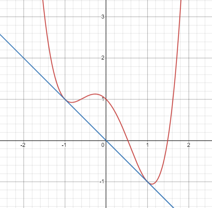
The parameter \(\gamma\) \((0<\gamma<1)\) corresponds to the fraction of blocks that would have a density \(\rho_1\) in the segregated state. This condition means that the value of the potential \(\Phi\) is lower for the segregated state than the homogeneous state (see Exercise 3.4.1). Such densities can be located geometrically as points of bitangency [Bertin 2021] (see the Figure below and Exercise 3.4.2).
Exercises#
Exercises
3.4.1. Show that in equilibrium the maximum likelihood configurations of densities \((\rho_1,...,\rho_Q)\) minimizes the potential function (‘free energy’) \(\Phi(\rho_1,...,\rho_Q)\) defined as
3.4.2. Find a line which is tangent to the quartic \(y=f(x)=x^4-2x^2-x+1\) at two different points \(P=(p,f(p))\) and \(Q=(q,f(q))\), Sketch the quartic and bi-tangent line.