Preview

Introduction

Calculus as we know it today would not have been developed without the Cartesian coordinate system and analytric geometry. Isaac Newton (1642-1727) attributed his success to "standing on the shoulders of giants" such as Descartes (1596-1650). In this section we explore how a concept as simple as graphing straight lines in a Cartesian plane is helpful in analyzing a budgeting problem called the "Two Commodity Model" [Vali 2014]. The simple idea that changing the coefficients in a linear relation will affect its graph (a simple example of "sensitivity analysis") becomes important when considering changes in unit prices and also in total budget amounts.

Reference: Vali, Shapor, 2014. Principles of Mathematical Economics. Paris: Atlantis Press.

Show code cell source Hide code cell source

import pandas as pd
import numpy as np
import matplotlib.pyplot as plt

7.2. Linear Systems and the Two-commodity Model

Two-commodity model

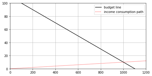
Suppose a household consumer is budgeting for two types of goods, necessities and luxuries. Let \(X\) denote the units of necessities and \(Y\) denote the units of luxuries. We let \(c_X\) denote the cost per unit of necessity and \(c_Y\) the cost per unit of luxury. If the total monthly budget is \(B\), then the budget equation is

\[ c_X X + c_Y Y = B. \]

Let \(r=\frac{Y}{X}\) be the ratio of units of luxury to units of necessities. Then the income consumption path is the line

\[ \frac{Y}{X}=r \Rightarrow Y=rX. \]

The equilibrium bundle is defined to be the point of intersection between the budget equation and the income consumption path.

Example

Find the equilibrium bundle if \(c_X=10,\) \(c_Y=100,\) \(B=11000\), and \(r=\frac{1}{100}.\)

Solution. In this case, the equilibrium bundle is the solution to the linear system

\[ 10X+100Y=11000 \Rightarrow Y=\frac{1}{100} X. \]

This system is easily solved to yield the equilibrium bundle (1000,10).

Here we plot the original budget constraint line and income consumption path.

Show code cell source Hide code cell source

cx=10  #unit price for necessities
cy=100  #unit price for luxuries
B=11000 #budget
x = np.linspace(0,1200,1000)
y_budget= (B-cx*x)/cy  #budget line
r=1/100 #ratio of luxuries to necessities
y_consump= r*x  #income consumption path
plt.figure(figsize=(8, 4))
plt.plot(x,y_budget,color='k',label="budget line")
plt.plot(x,y_consump,color='r',linestyle=":",label="income consumption path")
plt.xlim((0.,1200.))
plt.ylim((0,100.))
plt.grid()
plt.legend()
plt.show()

Sensitivity Analysis

A sensitivity analysis examines how a model is affected when one or more of its parameters are changed. For example, suppose due to inflation the cost per unit of necessity (\(c_X=10\)) and luxury \(c_Y=100\) both increase by 10%. Then the new budget equation is \(11X+110Y=11000\) and the new equilibrium bundle is approximately (909,9.1). This makes sense since higher unit prices mean less units of each type of item can be purchased.

Show code cell source Hide code cell source

x = np.linspace(0,1200.)
cx=10
cy=100
B=11000
y_budget= (B-cx*x)/cy
r=1/100
y_consump= r*x
cx1=11  #10% increase in necessity unit price
cy1=110 #10% increase in luxury unit price
y_budget1a= (B-cx1*x)/cy1
plt.figure(figsize=(8, 4))
plt.plot(x,y_budget,color='k',label = "Original budget")
plt.plot(x,y_budget1a,color='b',linestyle="-.",label = "10% increase in unit prices")
plt.plot(x,y_consump,color='r',linestyle=":",label="Income consumption path")
plt.xlim((0.,1200.))
plt.ylim((0,60.))
plt.xlabel("x=Units of Necessities")
plt.ylabel("y=Units of Luxuries")
plt.legend()
plt.grid()
plt.savefig("budget.png")
plt.show()
:::

Exercises

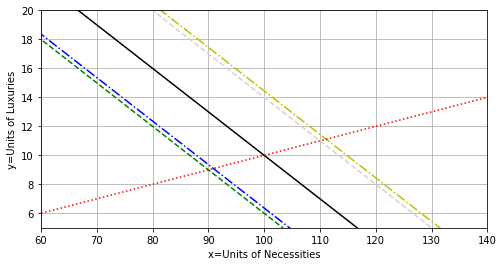
The following questions will compare the effect of increasing the budget vs. decreasing unit prices and also decreasing the budget vs. increasing the unit prices. Suppose that the monthly budget is $4,000 and the unit price for necessities is $30 and for luxuries it is $100.

1. Determine the equilibrium bundle if the ratio of necessities to luxuries is 10 to 1.

2. Which has the greater impact on the bundle: A 10% decline in budget or a 10% increase in unit prices?

3. Which has the greater impact on the bundle: A 10% increase in budget or a 10% decrease in unit prices?

4. Explain your answers to the above using the figure below.

Reference Vali, Shapor, 2014. Principles of Mathematical Economics. Paris: Atlantis Press.

Show code cell source Hide code cell source

x = np.linspace(0,1200.)
cx=30
cy=100
B=4000
y_budget= (B-cx*x)/cy
r=1/10
y_consump= r*x

cx1=33  #10% increase in necessity unit price
cy1=110 #10% increase in luxury unit price
y_budget1a= (B-cx1*x)/cy1

B1=3600 #10% decrease in budget 
y_budget1b= (B1-cx*x)/cy

cx2=27 #10% decrease in necessity unit price
cy2=90 #10% decrease in luxury unit price
y_budget2a= (B-cx2*x)/cy2

B2=4400  #10% increase in budget
y_budget2b= (B2-cx*x)/cy

plt.figure(figsize=(8, 4))
plt.plot(x,y_budget,color='k',label = "Original budget")
plt.plot(x,y_budget1a,color='b',linestyle="-.",label = "10% increase in unit prices")
plt.plot(x,y_budget1b,color='g',linestyle="--",label = "10% decrease in budget")
plt.plot(x,y_budget2a,color='y',linestyle="-.",label = "10% decrease in unit prices")
plt.plot(x,y_budget2b,color='lightgray',linestyle="--",label = "10% increase in budget")
plt.plot(x,y_consump,color='r',linestyle=":",label="Income consumption path")
plt.xlim((60.,140.))
plt.ylim((5,20.))
plt.xlabel("x=Units of Necessities")
plt.ylabel("y=Units of Luxuries")
#plt.legend()
plt.grid()
plt.savefig("budgetex.png")
plt.show()