11.3. First-Order Differential Equations#
Note
In this chapter, methods will be given for solving first-order differential equations. Remember that first-order means that the first derivative of the unknown function is the highest derivative appearing in the equation.
11.3.1. Separable First-Order Differential Equations#
A first order differential equation is called separable if it can be written as \(\frac{dx}{dt} = f(x) \cdot g(t)\), that is, the independent variable and the dependent variable of the differential equation can be separated from one another.
Example
\(y' = x^3\) is a separable differential equation.
\(\frac{dx}{dt} = kx^2\sin(t)\) is a separable differential equation.
\(y'(x) = x^2 -3y\) is not a separable differential equation.
\(\frac{dx}{dt}\cdot t -3xt^2 = 7t^2\) is a separable differential equation. In particular, this can be rewritten as \(\frac{dx}{dt} = (7+3x)t\).
Given a separable differential equation \(\frac{dx}{dt} = f(x) \cdot g(t)\), we can solve it with the following procedure.
Separate the variables: \(\frac{1}{f(x)}dx = g(t)dt\)
Note: \(\frac{dx}{dt}\) is not a fraction, but this process can be done because we are implicitly applying the chain rule for multivariate functions.
Integrate both sides with respect to the appropriate variable: \(\displaystyle{\int \frac{1}{f(x)}dx = \int g(t)dt}\).
Write the solution in the form \(F(x) = G(t)+C\), where \(F'(x) = \frac{1}{f(x)}\) and \(G'(t)=g(t)\).
If possible, solve the equation explicitly for the dependent variable, in this case \(x\).
Example
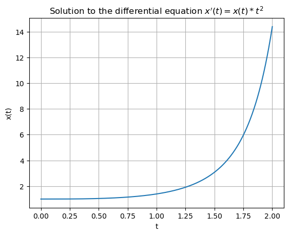
Find the explicit general solution to the differential equation \(\frac{dx}{dt} = xt^2\).
Separate: \(\frac{1}{x} dx = t^2 dt\)
Integrate: \(\displaystyle{\int \frac{1}{x} dx = \int t^2 dt}\)
\(\ln|x| = \frac{1}{3}t^3 + C\) \(\rightarrow\) Note: This is the implicit solution to the differential equation.
Solve for the Dependent Variable:
Show code cell source
from sympy import Function, dsolve, Eq, Derivative, symbols
from sympy.abc import t

# Define the unknown function x(t)
x = Function('x')

# Define the differential equation x'(t) = x(t)*t^2
diff_eq = Eq(Derivative(x(t),t), x(t)*t**2)

# Solve the differential equation
solution = dsolve(diff_eq)

print(solution)
Eq(x(t), C1*exp(t**3/3))
Show code cell source
import numpy as np
from scipy.integrate import odeint
import matplotlib.pyplot as plt

# Define the function for the differential equation
def dx_dt(x, t):
    return x*t**2

# Define the time range over which to solve the differential equation
t = np.linspace(0, 2, 1000)

# Define the initial condition x(0)=1
x0 = 1

# Solve the differential equation
x = odeint(dx_dt, x0, t)

# Plot the solution
plt.plot(t, x)
plt.xlabel('t')
plt.ylabel('x(t)')
plt.title("Solution to the differential equation $ x'(t) = x(t)*t^2 $")
plt.grid(True)
plt.show()
Example
Find the explicit solution to the initial value problem \(\frac{dW}{ds} = \frac{2s \cos^2(W)}{s^2-1}\) where \(W(0)=0\).
Separate: \(\frac{1}{\cos^2(W)} dW = \frac{2s}{s^2-1} ds\)
Integrate: \(\displaystyle{\int \sec^2(W) dW = \int \frac{2s}{s^2-1} ds}\)
\(\tan(W) = \ln|s^2-1| + C\) \(\rightarrow\) Note: This is the implicit solution to the differential equation.
Solve for the Dependent Variable:
Use Initial Condition \(W(0)=0\):
Explicit Solution: \(W = \arctan(\ln|s^2-1|)\)
11.3.2. Linear First-Order Differential Equations#
A first order differential equation is called linear if it can be written as \(a_1(t)\frac{dx}{dt} + a_0(t)x= g(t)\). The equation is linear in the dependent variable, in this case \(x\), and its derivative; the coefficient functions \(a_1(t)\), \(a_0(t)\), and \(g(t)\) can be any function involving \(t\).
Example
\(y' + ye^x = \tan(t)\) is a linear differential equation.
\(x\frac{dx}{dt} = kx^2\sin(t)\) is not a linear differential equation because of the \(x \frac{dx}{dt}\) term.
\(x'(t) = x^2 -3t\) is not a linear differential equation because of the \(x^2\) term.
\(\frac{dx}{dt}\cdot t -3xt^2 = 7t^2\) is a linear differential equation. In particular, this can be rewritten as \(t\frac{dx}{dt} -3t^2x = 7t^2\).
A first-order linear differential equation is said to be in standard form if it is written in the form \(\frac{dx}{dt} + p(t)x = q(t)\). In other words, if the coefficient on the first derivative is \(1\). Note that any first-order linear differential equation can be written in standard form by performing simple algebra.
If \(q(t)=0\), we say that the differential equation is homogeneous. If \(q(t) \neq 0\), we say that the differential equation is nonhomogeneous. Note that if a first order differential equation is both linear and homogeneous, then it is also separable. You will be asked to show why in the exercises.
We will now develop a strategy for solving first-order linear differential equations. The basic idea is that we will multiply by a positive function that simplifies the left hand side of the differential equation. We must choose a positive function in order to preserve the solutions to the differential equation.
Given a first-order linear differential equation in standard form \(x' + p(t)x = q(t)\), the integrating factor for the differential equation is the function \(\mu(t) = e^{P(t)}\) where \(P(t)\) is any antiderivative of \(p(t)\), that is, \(P'(t)=p(t)\). The integrating factor is the positive function that we will multiply our differential equation by. So what is the significance of multiplying by the integrating factor?
Consider \(x' + p(t)x = q(t)\).
Multiply by \(\mu(t) = e^{P(t)}\), which yields \(\mu(t)x' + \mu(t)p(t)x = \mu(t)q(t)\)
Observe \(\mu'(t) = e^{P(t)}P'(t) = e^{P(t)}p(t) = \mu(t)p(t)\).
Rewrite \(\mu(t)x' + \mu(t)p(t)x = \mu(t)q(t)\) as \(\mu(t)x' + \mu'(t)x = \mu(t)q(t)\).
Observe \(\frac{d}{dt}\left( \mu(t)x(t) \right) = \mu(t)x'(t) + \mu'(t)x(t)\).
Rewrite \(\mu(t)x' + \mu'(t)x = \mu(t)q(t)\) as \(\frac{d}{dt}\left( \mu(t)x(t) \right) = \mu(t)q(t)\).
Integrate \(\displaystyle{\int \frac{d}{dt}\left( \mu(t)x(t) \right) dt = \int \mu(t)q(t) dt}\).
\(\displaystyle{\mu(t)x(t) = \int \mu(t)q(t) dt}\)
Solve for the dependent variable
\(x(t) = \displaystyle{\frac{1}{\mu(t)} \int \mu(t)q(t) dt}\).
Note we have no guarantee that we can integrate \(\int \mu(t)q(t) dt\), but if we can we are able to solve first-order linear differential equations.
Example
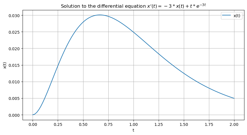
Find the general solution to the differential equation \(\frac{dx}{dt} + 3x = te^{-3t}\).
Note: This differential equation is in standard form so we can proceed by finding the integrating factor.
Multiply by \(\mu(t) = e^{\int 3 dt} = e^{3t}\).
Observe \(\frac{d}{dt}(e^{3t}\cdot x(t)) = e^{3t}x'(t)+3e^{3t}x(t)\).
Rewrite \(e^{3t}x'(t)+3e^{3t}x(t) = t\) as \(\frac{d}{dt}(e^{3t}\cdot x(t)) = t\).
Integrate \(\displaystyle{\int \frac{d}{dt}(e^{3t}\cdot x(t)) dt = \int t dt}\).
Solve for the dependent variable.
Show code cell source
import sympy as sp

# Define the variables
t = sp.symbols('t')
x = sp.Function('x')

# Define the differential equation x'(t) = -3*x(t) + t*exp(-3t)
diff_eq = sp.Eq(x(t).diff(t), -3*x(t) + t*sp.exp(-3*t))

# Solve the differential equation
solution = sp.dsolve(diff_eq)

print(solution)
Eq(x(t), (C1 + t**2/2)*exp(-3*t))
Show code cell source
import sympy as sp
import numpy as np
import matplotlib.pyplot as plt

# Define the symbols
t = sp.symbols('t')
x = sp.Function('x')

# Define the differential equation
diff_eq = sp.Eq(x(t).diff(t), -3*x(t) + t*sp.exp(-3*t))

# Solve the differential equation
solution = sp.dsolve(diff_eq)

# Create a lambdified function that can be used in numpy from the solution
# Assuming C1 = 0
f = sp.lambdify(t, solution.rhs.subs('C1', 0), 'numpy')

# Generate t values
t_values = np.linspace(0, 2, 100)

# Generate y values
y_values = f(t_values)

# Plot the solution
plt.figure(figsize=(10,5))
plt.plot(t_values, y_values, label='x(t)')
plt.title('Solution to the differential equation $ x\'(t) = -3*x(t) + t*e^{-3t} $')
plt.xlabel('t')
plt.ylabel('x(t)')
plt.legend()
plt.grid(True)
plt.show()
11.3.3. Slope Fields#
Note we still do not know how to solve every first-order linear differential equation. For example, \(y' = x(x^2-y^2)\) is neither separable or linear. However, even if we cannot solve a differential equation, it is still possible to get qualitative information about the solution.
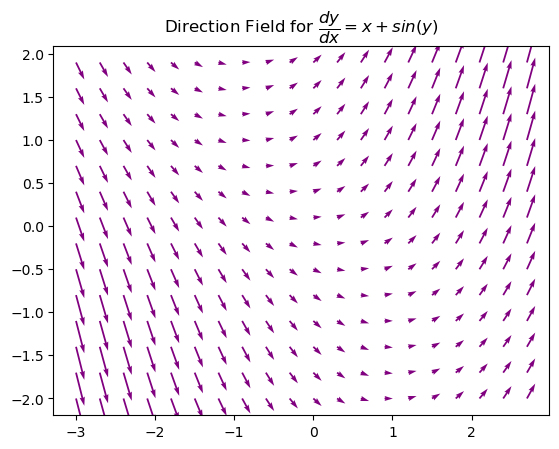
Consider the first-order differential equation \(\frac{dx}{dt} = f(t,x)\). If we evaluate \(f(t,x)\) at a set of grid points, we can then draw short vectors that represent the slope of the solution \(x(t)\) at those points. If we look at this grid of vectors at many points, we can get an idea of what the solution, \(x(t)\), looks like. This grid of vectors is called a slope field or direction field.
To draw a direction field, you can simply evaluate the differential equation at various points and plot the resulting vectors. For example, using the equation \(y' = x(x^2-y^2)\), if you plug in the point (0,0), you see that the slope (\(y'\)) is \(0\) at that point, so you can draw a short vector of \(0\) slope at the origin. In fact, whenever \(x = 0\), the slope is \(0\), so along the y-axis, there will be short horizontal (\(0\) slope) vectors at every y-value. This process can be repeated for a set of sample points to create a graph that tells us about the behavior of solutions to a first order equation.
Direction fields can also be plotted using electronically, as demonstrated below.
Example
Plot a direction field for \(y'(x) = x + \sin(y)\).
Show code cell source
import numpy as np
import matplotlib.pyplot as plt

nx, ny = .3, .3
x = np.arange(-3,3,nx)
y = np.arange(-2,2,ny)

#Create a rectangular grid with points
X,Y = np.meshgrid(x,y)

#Define the functions
dy = X + np.sin(Y)
dx = np.ones(dy.shape)

#Plot
plt.quiver(X,Y,dx,dy,color='purple')
plt.title('Direction Field for $\dfrac{dy}{dx} = x + sin(y) $')
plt.show()
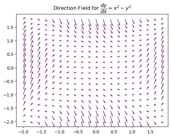
Example
Plot a direction field for \(y'(x) = x^2 - y^2\).
Show code cell source
import numpy as np
import matplotlib.pyplot as plt

#Take some time to play around with the various parameters and see how it impacts the slope-field that is produced.
nx, ny = .2, .2
x = np.arange(-2,2,nx)
y = np.arange(-2,2,ny)

#Create a rectangular grid with points
X,Y = np.meshgrid(x,y)

#Define the functions
dy = X**2 -Y**2
dx = np.ones(dy.shape)

#Plot
plt.quiver(X,Y,dx,dy,color='purple')
plt.title('Direction Field for $ \dfrac{dy}{dx} = x^2 -y^2 $')
plt.show()
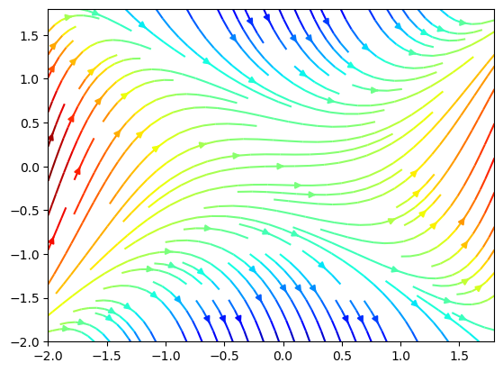
Example
Plot a direction field for \(y'(x) = x^2 - y^2\).
Show code cell source
import numpy as np
from scipy.integrate import odeint
import matplotlib.pyplot as plt

#Take some time to play around with the various parameters and see how it impacts the slope-field that is produced.
nx, ny = .2, .2
x = np.arange(-2,2,nx)
y = np.arange(-2,2,ny)

#Create a rectangular grid with points
X,Y = np.meshgrid(x,y)

#Define the functions
dy = X**2 -Y**2
dx = np.ones(dy.shape)

#Plot
plt.quiver(X,Y,dx,dy,color='purple')
plt.title('Direction Field for $ \dfrac{dy}{dx} = x^2 -y^2 $')
plt.show()

#You can also use the streamlines of the field to give a nice impression of the flow and color the curves.
plt.streamplot(X,Y,dx, dy, color=dy, density=1., cmap='jet', arrowsize=1)
plt.show()
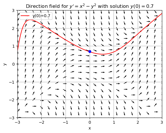
You may use the following code to plot a direction field for \(y'(x) = x^2-y^2\) and a particular solution curve given an initial condition.
Show code cell source
import numpy as np
from scipy.integrate import odeint
import matplotlib.pyplot as plt

# Define the function for the differential equation
def dy_dx(y, x):
    return x**2 - y**2

# Generate a grid of points on which to evaluate the direction field
x = np.linspace(-3, 3, 20)
y = np.linspace(-3, 3, 20)

X, Y = np.meshgrid(x, y)
U = 1
V = dy_dx(Y, X)
N = np.sqrt(U**2 + V**2)  # Normalize arrow length
U /= N
V /= N

# Plot the direction field
plt.quiver(X, Y, U, V, angles='xy')

# Solve the differential equation for the initial condition y(0)=1
x = np.linspace(-3, 3, 100)
y0 = .7  # initial condition
y = odeint(dy_dx, y0, x)

# Plot the solution on the direction field
plt.plot(x, y, 'r', label='y(0)=0.7')

# Plot the point (0,0.7)
plt.plot(0, .7, 'bo')  # 'bo' means blue dot

plt.xlim([-3, 3])
plt.ylim([-3, 3])
plt.xlabel('x')
plt.ylabel('y')
plt.grid(True)
plt.legend()
plt.title("Direction field for $ y'=x^2-y^2 $ with solution $ y(0)=0.7 $")
plt.show()
Example
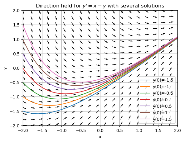
Plot a direction field for \(y'(x) = x - y\) with multiple solution curves.
Show code cell source
import numpy as np
from scipy.integrate import odeint
import matplotlib.pyplot as plt

# Define the function for the differential equation
def dy_dx(y, x):
    return x - y

# Generate a grid of points on which to evaluate the direction field
x = np.linspace(-2, 2, 20)
y = np.linspace(-2, 2, 20)

X, Y = np.meshgrid(x, y)
U = 1
V = dy_dx(Y, X)
N = np.sqrt(U**2 + V**2)  # Normalize arrow length
U /= N
V /= N

# Plot the direction field
plt.quiver(X, Y, U, V, angles='xy')

# Solve the differential equation for various initial conditions and plot
x = np.linspace(-2, 2, 100)
initial_conditions = [-1.5, -1, -0.5, 0, 0.5, 1, 1.5]  # change as desired
for y0 in initial_conditions:
    y = odeint(dy_dx, y0, x)
    plt.plot(x, y, label=f'y(0)={y0}')

plt.xlim([-2, 2])
plt.ylim([-2, 2])
plt.xlabel('x')
plt.ylabel('y')
plt.grid(True)
plt.legend()
plt.title("Direction field for $ y'=x-y $ with several solutions")
plt.show()
You may also use the following code to plot a direction field for \(y'(x) = x-y\) and a single solution curve. Notice that there is a slider which allows you to adjust the initial condition and see different solution curves based on your choice of initial condition.
Note
If you are reading this textbook in a format that does not allow this code cell to be executed (such as a webpage or a PDF), please download the original Jupyter Notebook or launch it in Binder to engage with this interactive resource.
Show code cell source
import numpy as np
from scipy.integrate import odeint
import matplotlib.pyplot as plt
from ipywidgets import interact, FloatSlider

# Define the function for the differential equation
def dy_dx(y, x):
    return x - y

# Define the x range and initial conditions
x = np.linspace(-2, 2, 100)

@interact
def plot_solution_curve(y0=FloatSlider(min=-2.0, max=2.0, step=0.1, value=0.0)):

    # Generate a grid of points on which to evaluate the direction field
    x_grid = np.linspace(-2, 2, 20)
    y_grid = np.linspace(-2, 2, 20)

    X, Y = np.meshgrid(x_grid, y_grid)
    U = 1
    V = dy_dx(Y, X)
    N = np.sqrt(U**2 + V**2)  # Normalize arrow length
    U /= N
    V /= N

    # Plot the direction field
    plt.quiver(X, Y, U, V, angles='xy')

    # Solve the differential equation for the given initial condition
    y = odeint(dy_dx, y0, x)

    # Plot the solution on the direction field
    plt.plot(x, y, 'r', label=f'y(0)={y0}')

    plt.xlim([-2, 2])
    plt.ylim([-2, 2])
    plt.xlabel('x')
    plt.ylabel('y')
    plt.grid(True)
    plt.legend()
    plt.title("Direction field for y'=x-y with adjustable initial condition")
    plt.show()
11.3.4. Autonomous Equations#
A first-order differential equation of the form \(\frac{dx}{dt} = f(x)\) is called autonomous, that is, a differential equation where only the dependent variable appears. We can always solve these because they are always separable. In particular, we can always rewrite the differential equation as \(\displaystyle{\int \frac{1}{f(x)} dx = \int dt}\) assuming \(f(x) \neq 0\). But it can sometimes be very difficult to do so.
It turns out that autonomous differential equations are nice in that they have constant solutions. In particular, \(x(t)=c\) is a solution if \(x'(t) = \frac{dc}{dt} = 0 = f(x(t)) = f(c)\). These are the trivial solutions we would lose when dividing by zero when handling it as a separable differential equation.
An equilibrium solution of an autonomous differential equation is a constant solution to the differential equation. In other words, if \(f(c)=0\), then \(x(t)=c\) is an equilibrium solution of \(x'(t)=f(x)\).
Example
Find the equilibrium solutions of \(x'(t) = x^2 - 9\).
\(x'(t)=0\)
\(x^2-9=(x-3)(x+3)=0\)
So \(x(t) = -3\) and \(x(t)=3\) are the equilibrium solutions.
*Note: \(\displaystyle{\int \frac{1}{x^2-9} dx = \int dt}\) would not have recovered these solutions.
Given the equilibrium solutions of an autonomous differential equation, we can make a phase line to analyze the behavior of the solution.
Example
Draw a phase line and determine where the solutions of the differential equation \(y'(x) = y(y-1)^2(y-2)\) are increasing and decreasing.
First we must find the equilibrium solutions, which means we must solve \(y'(x)=0\). This means \(y(y-1)^2(y-2)=0\). So \(y(x)=0\), \(y(x)=1\), and \(y(x)=2\) are the equilibrium solutions. To draw a phase line, see the code below.
Show code cell source
import numpy as np
import matplotlib.pyplot as plt

# Function for the autonomous differential equation
def f(y):
    return y * (y - 1)**2 * (y - 2)

# Identify the critical points (where dy/dx = 0)
critical_points = [0, 1, 2]

# Create the figure and axis
fig, ax = plt.subplots()

# Plot the phase line at x = 0 with markers at the critical points
for point in critical_points:
    if f(point - 0.01) > 0 > f(point + 0.01):
        ax.plot(0, point, 'go')  # Stable points in green
    elif f(point - 0.01) < 0 < f(point + 0.01):
        ax.plot(0, point, 'ro')  # Unstable points in red
    else:
        ax.plot(0, point, 'yo') # Semi-stable point in yellow

# Draw arrows indicating direction of movement
arrow_properties = dict(facecolor='black', width=0.075, head_width=.3, head_length=.3)  # Decrease head_width to make arrows skinnier

check_points = [-0.5, 0.5, 1.5, 2.5]

# Check below the lowest critical point separately
if f(check_points[0]) > 0:
    ax.arrow(0, (check_points[0] - 1)/1.8, 0, 0.3, **arrow_properties)  # Pointing up if derivative is positive
else:
    ax.arrow(0, (check_points[0] - 1)/1.8, 0, -0.3, **arrow_properties)  # Pointing down if derivative is negative

for i in range(len(critical_points) - 1):
    if f(check_points[i+1]) > 0:
        ax.arrow(0, (critical_points[i] + critical_points[i+1])/1.7, 0, 0.3, **arrow_properties)  # Pointing up if derivative is positive
    else:
        ax.arrow(0, (critical_points[i] + critical_points[i+1])/1.7, 0, -0.3, **arrow_properties)  # Pointing down if derivative is negative

# Check above the highest critical point separately
if f(check_points[-1]) > 0:
    ax.arrow(0, (critical_points[-1] + 3)/2.1, 0, 0.3, **arrow_properties)  # Pointing up if derivative is positive
else:
    ax.arrow(0, (critical_points[-1] + 3)/2.1, 0, -0.3, **arrow_properties)  # Pointing down if derivative is negative

# Set the y-axis limits
plt.ylim(-1.1, 3.1)
# Set the x-axis limits
plt.xlim(-0.5, 0.5)

# Label the y-axis
plt.ylabel('y')

# Title of the plot
plt.title('Phase Line Plot')

# Remove the x-axis
plt.gca().axes.get_xaxis().set_visible(False)

# Show the plot
plt.show()
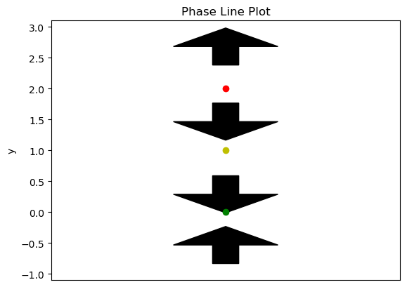
Notice that this tells us that a solution to the previous differential equation would have to be increasing on the interval \((-\infty,0)\) or decreasing on \((0,1)\) or decreasing on \((1,2)\) or increasing on \((2,\infty)\).
In addition it allows us to classify the stability of our equilibrium solutions. An equilibrium solution \(x(t)=c\) is stable if solutions whose initial value is near \(c\) stays near \(c\) as the independent variable increases. An equilibrium solution \(x(t)=c\) is unstable if solutions whose initial value is near \(c\) goes away from \(c\) as the independent variable increases. An equilibrium solution is considered semi-stable if both cases occur (one in the region above and one in the region below). We can see an example of each type of equilibrium in the above example. In particular, \(x(t)=0\) is stable, \(x(t)=1\) is semi-stable, and \(x(t)=2\) is unstable. Alternatively, a stable solution can be referred to as a sink, an unstable solution as a source, and a semi-stable solution as a node.
It turns out that if we know that there is a unique solution to the autonomous initial-value problem \(\frac{dx}{dt} = f(x)\) where \(x(t_0)=x_0\), then we know a few more things about the solution. Namely,
The equilibrium points divide the region \(\mathbb{R}^2\) plane into regions. A solution cannot pass between regions and the initial value will determine which region a particular solution is in.
The solution \(x(t)\) is increasing/decreasing everywhere inside a particular region because \(f(x)\) is either positive or negative everywhere in a region.
The limit of a solution \(x(t)\) as \(t \rightarrow \pm \infty\) is one of the boundaries of that region.
11.3.5. Exercises#
Exercises
Determine if the following first-order differential equations are linear, separable, both, or neither.
\(\frac{dy}{dx} = y + x\)
\(\sqrt{y} + 2\frac{dy}{dx} = e^{x}\)
\(\sqrt{y}\frac{dy}{dx} = e^{x}\)
\(\frac{dy}{dx} = x+5\)
Find the explicit solution to the differential equation \(y'(x) = y+5\).
Find the explicit solution to the differential equation \(W'(s) = s+sW^2\).
Find the explicit solution to the initial value problem \(y'(t) = ty\) where \(y(0)=3\).
Find the explicit solution to the initial value problem \(x'(t) = x\sin(t)\) where \(x(0)=1\).
Show that if a first order differential equation is both linear and homogeneous, then it is also separable.
Find the solution to the differential equation \(\frac{dP}{dt} = \frac{2P}{t} + t^2\sec^2(t)\).
Find the solution to the initial value problem \(xy' + y = \sin(x)\), where \(y(\pi)=0\).
Plot a direction field for \(y'(x) = y+x\).
Plot a direction field for \(y'(x) = xy\).
Find the equilibrium solutions of \(y'(x) = \sin(y)\).
Draw a phase line and determine where a solution of the differential equation \(\frac{dT}{dt} = (T+1)T(T-3)^2\) is increasing and decreasing. Then classify the stability of each equilibrium point.