7.10. Partial Derivatives and OLS Regression#
Ordinary least squares (OLS) regression of 2-dimensional data is an important concept in data analysis. Given a collection of data points
the goal is to find a line \(y=mx+b\) (called the OLS regression line) that best fits the data in the sense that it minimizes the sum of square vertical separations between the data points and the line:
The optimal values of \(m\) and \(b\) minimize \(S(m,b)\), and hence may be obtained using a system of two equations and 2 unknowns:
Example
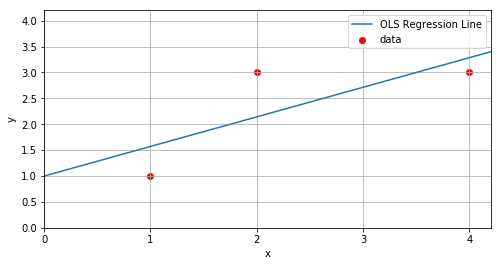
Consider the data values (1,1), (2,3), and (4,3). In this case,
This gives rise to the system
The system is equivalent to
We can solve this system by multiplying the first equation through by 3, and the second equation through by 7
Subtracting the second equation from the first equation gives
We find \(b\) by back substitution:
The plot below shows the OLS regression line \(y=\frac{4}{7}x+1\) together with the three data points.
Show code cell source
import matplotlib.pyplot as plt
import numpy as np
plt.figure(figsize=(8, 4))
plt.xlim((0,4.2))
plt.ylim((0,4.2))
#--plot the data points-----
x=[1,2,4] #(x coordinates of the data)
y=[1,3,3] #(y-coordinates of the data)
plt.scatter(x,y,color='r',label='data')
#--plot the OLS regression line-----
m=4/7
b=1
xreg=np.linspace(0,5,50)
yreg=m*xreg+b
plt.plot(xreg,yreg,label="OLS Regression Line")
plt.gca().set_xticks(np.arange(0,5,1))
plt.grid()
plt.legend()
plt.xlabel("x")
plt.ylabel("y")
plt.show()
7.10.1. Exercises#
Exercises
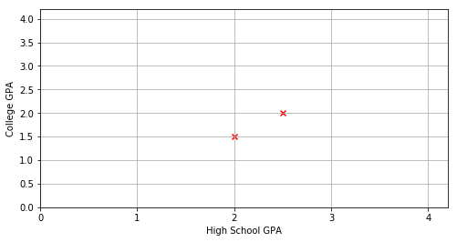
A college admissions officer has compiled the following data relating 8 students’ high school and college GPA:
GPA |
||||||||
|---|---|---|---|---|---|---|---|---|
High School GPA: |
2.0 |
2.5 |
3.0 |
3.0 |
3.5 |
3.5 |
4.0 |
4.0 |
College GPA: |
1.5 |
2.0 |
2.5 |
3.5 |
2.5 |
3.0 |
3.0 |
3.5 |
Complete the plot of this data and then guess the value of \(m\) and \(b\) for the least squares regression line \(y=mx+b\). (Use your guess to check that your answer to problem 2 is reasonable).
Show code cell source
import matplotlib.pyplot as plt
import numpy as np
plt.figure(figsize=(8, 4))
plt.xlim((0,4.2))
plt.ylim((0,4.2))
hs=[2.0,2.5]
col=[1.5,2.0]
plt.scatter(hs,col,color='r',marker='x')
plt.gca().set_xticks(np.arange(0,5,1))
plt.grid()
plt.xlabel("High School GPA")
plt.ylabel("College GPA")
plt.show()
Exercises (continued)
Use calculus to find the least squares regression line \(y=mx+b\).
Use the second derivative test to verify the choice of \(m\) and \(b\) in problem 2 that gives a minimum for the sum of squares \(S(m,b)\).
Use the regression line to predict the college GPA’s:
GPA |
|||
|---|---|---|---|
High School GPA: |
2.0 |
3.0 |
4.0 |
College GPA: |